Gravitino, graviton and axino production in the MSSM#
[1]:
#import the autotherm modules
from analytical.controller import *
from numerical.manipulate import *
#not needed as it is already pulled my manipulate, but reimporting it fixes
#syntax highlighting in vscode
import numpy
#import matplotlib too
import matplotlib.pyplot as plt
Gravitino and graviton production in the MSSM#
For gravitino production, the relevant part of the config file mssm_gravitino.cfg is as follows
[Model]
modelpath = /Users/jacopo/NextCloud/AUTOTHERM/autotherm/analytical/models/MSSM.fr
# Symbol for the Lagrangian in the model file
lagrangian = LtotsuperG
# "Name" of the particle whose production rate must be computed
# Unused for now, but still required. Put something like T[1]
produced = F[11]
# List of the particles in the thermal bath (or leave empty for SM assumption)
# Unused for now, but still required.
inbath = S[2]+ -S[2]+ S[3]+ -S[3]+ S[4]+ -S[4]+ S[5]+ -S[5]+ S[6]+ -S[6]+ S[7]+ -S[7]+ F[6]+ -F[6]+ F[7]+ -F[7]+ F[8]+ -F[8]+ F[9]+ -F[9]+ F[10]+ -F[10]+
assumptions = Element[ht,Reals], Element[kappa,Reals], g1>0, g2>0, g3>0
replacements =
includeSM = no
noneq = kappa
#comma-separated list of particles to be treated with a flavor expansion
flavorexpand =
To produce the graviton, we set produced = T[1] rather than F[11] in the block above, so as to obtain mssm_grav.cfg
[ ]:
gravitondict=analytical_pipeline("../../MyModels/mssm_grav/mssm_grav.cfg")
[3]:
graviton=NumRate(*gravitondict,2)
k=numpy.logspace(numpy.log10(0.1),numpy.log10(12.5),100)
Gravitino determination using the goldstino rules
[ ]:
gravitinodict=analytical_pipeline("../../MyModels/mssm_gravitino/mssm_gravitino.cfg")
gravitino=NumRate(*gravitinodict,1)
let us inspect the gravitino results and put the matrix elements squared in a compact form
[8]:
from IPython.display import display, Markdown
out=""
s = sympy.Symbol("s")
t = sympy.Symbol("t")
u = sympy.Symbol("u")
g1 = sympy.Symbol("g1")
g2 = sympy.Symbol("g2")
g3 = sympy.Symbol("g3")
ht = sympy.Symbol("ht")
cy = sympy.Symbol(r"C_\mathrm{Yukawa}")
cg = sympy.Symbol(r"C_\mathrm{gauge}")
kappa=sympy.Symbol("kappa")
for key, item, in gravitinodict[0].items():
    sitem=sympy.simplify(sympy.sympify(item))
    sitemsubst= sympy.simplify(sitem.subs(ht*ht,(cy-11*g1**2-21*g2**2-48*g3**2)/9).subs(g1*g1,(cg-27*g2**2-72*g3**2)/11))
    sitemsubstcollect=0
    for exprtemp in sympy.factor(sitemsubst.expand().as_independent(cy)).subs(t+u,-s)\
        .subs(2*t*t+2*t*u,2*t*t+(s*s-t*t-u*u)).subs(t*t+2*t*u,t*t+(s*s-t*t-u*u)).subs(t*t+t*u,t*t+(s*s-t*t-u*u)/2):
        sitemsubstcollect += exprtemp.simplify()
    out+=f"-  $$ \\left\\vert \\mathcal{{M}}_\\psi({key[0]};{key[1]},{key[2]})\\right\\vert^2={sympy.latex(sitem).replace('ht^{2}',r'\vert h_t\vert^2')}$$\n or\n  $$ \\left\\vert \\mathcal{{M}}_\\psi({key[0]};{key[1]},{key[2]})\\right\\vert^2={sympy.latex(sitemsubstcollect)}$$\n"
    # display(sympy.pprint(sitem))
display(Markdown(out))
- \[\left\vert \mathcal{M}_\psi(-1;-1,-1)\right\vert^2=\frac{\kappa^{2} \left(11 g_{1}^{2} + 27 g_{2}^{2} + 72 g_{3}^{2}\right) \left(t^{2} + t u + u^{2}\right)^{2}}{s t u}\]
or
\[\left\vert \mathcal{M}_\psi(-1;-1,-1)\right\vert^2=\frac{C_\mathrm{gauge} \kappa^{2} \left(s^{2} + t^{2} + u^{2}\right)^{2}}{4 s t u}\] - \[\left\vert \mathcal{M}_\psi(1;-1,1)\right\vert^2=- \frac{\kappa^{2} \left(t^{2} \left(11 g_{1}^{2} + 27 g_{2}^{2} + 72 g_{3}^{2}\right) + t u \left(11 g_{1}^{2} + 27 g_{2}^{2} + 72 g_{3}^{2}\right) + \frac{3 u^{2} \left(11 g_{1}^{2} + 23 g_{2}^{2} + 56 g_{3}^{2} + 6 \vert h_t\vert^2\right)}{2}\right)}{u}\]
or
\[\left\vert \mathcal{M}_\psi(1;-1,1)\right\vert^2=- C_\mathrm{Yukawa} \kappa^{2} u - \frac{C_\mathrm{gauge} \kappa^{2} \left(s^{2} + t^{2}\right)}{2 u}\] - \[\left\vert \mathcal{M}_\psi(1;1,-1)\right\vert^2=- \frac{\kappa^{2} \left(\frac{3 t^{2} \left(11 g_{1}^{2} + 23 g_{2}^{2} + 56 g_{3}^{2} + 6 \vert h_t\vert^2\right)}{2} + t u \left(11 g_{1}^{2} + 27 g_{2}^{2} + 72 g_{3}^{2}\right) + u^{2} \left(11 g_{1}^{2} + 27 g_{2}^{2} + 72 g_{3}^{2}\right)\right)}{t}\]
or
\[\left\vert \mathcal{M}_\psi(1;1,-1)\right\vert^2=- C_\mathrm{Yukawa} \kappa^{2} t - \frac{C_\mathrm{gauge} \kappa^{2} \left(s^{2} + u^{2}\right)}{2 t}\] - \[\left\vert \mathcal{M}_\psi(-1;1,1)\right\vert^2=\frac{\kappa^{2} \left(\frac{t^{2} \left(33 g_{1}^{2} + 69 g_{2}^{2} + 168 g_{3}^{2} + 18 \vert h_t\vert^2\right)}{2} + 2 t u \left(11 g_{1}^{2} + 21 g_{2}^{2} + 48 g_{3}^{2} + 9 \vert h_t\vert^2\right) + \frac{u^{2} \left(33 g_{1}^{2} + 69 g_{2}^{2} + 168 g_{3}^{2} + 18 \vert h_t\vert^2\right)}{2}\right)}{s}\]
or
\[\left\vert \mathcal{M}_\psi(-1;1,1)\right\vert^2=C_\mathrm{Yukawa} \kappa^{2} s + \frac{C_\mathrm{gauge} \kappa^{2} \left(t^{2} + u^{2}\right)}{2 s}\]
the same can be done for the graviton matrix elements
[9]:
out=""
for key, item, in gravitondict[0].items():
    sitem=sympy.simplify(sympy.sympify(item))
    sitemsubst= sympy.simplify(sitem.subs(ht*ht,(cy-11*g1**2-21*g2**2-48*g3**2)/9).subs(g1*g1,(cg-27*g2**2-72*g3**2)/11))
    sitemsubstcollect=0
    for exprtemp in sympy.factor(sitemsubst.expand().as_independent(cy)).subs(t+u,-s)\
        .subs(2*t*t+2*t*u,2*t*t+(s*s-t*t-u*u)).subs(t*t+2*t*u,t*t+(s*s-t*t-u*u)).subs(t*t+t*u,t*t+(s*s-t*t-u*u)/2):
        sitemsubstcollect += exprtemp.simplify()
    out+=f"-  $$ \\left\\vert \\mathcal{{M}}_G({key[0]};{key[1]},{key[2]})\\right\\vert^2={sympy.latex(sitem).replace('ht^{2}',r'\vert h_t\vert^2')}$$\n or\n  $$ \\left\\vert \\mathcal{{M}}_G({key[0]};{key[1]},{key[2]})\\right\\vert^2={sympy.latex(sitemsubstcollect)}$$\n"
    # display(sympy.pprint(sitem))
display(Markdown(out))
- \[\left\vert \mathcal{M}_G(1;-1,-1)\right\vert^2=\frac{\kappa^{2} \left(t^{2} \left(33 g_{1}^{2} + 69 g_{2}^{2} + 168 g_{3}^{2} + 18 \vert h_t\vert^2\right) + 4 t u \left(11 g_{1}^{2} + 21 g_{2}^{2} + 48 g_{3}^{2} + 9 \vert h_t\vert^2\right) + u^{2} \left(33 g_{1}^{2} + 69 g_{2}^{2} + 168 g_{3}^{2} + 18 \vert h_t\vert^2\right)\right)}{s}\]
or
\[\left\vert \mathcal{M}_G(1;-1,-1)\right\vert^2=2 C_\mathrm{Yukawa} \kappa^{2} s + \frac{C_\mathrm{gauge} \kappa^{2} \left(t^{2} + u^{2}\right)}{s}\] - \[\left\vert \mathcal{M}_G(-1;-1,1)\right\vert^2=\frac{\kappa^{2} \left(t^{2} \left(- 33 g_{1}^{2} - 69 g_{2}^{2} - 168 g_{3}^{2} - 18 \vert h_t\vert^2\right) - 2 t u \left(11 g_{1}^{2} + 27 g_{2}^{2} + 72 g_{3}^{2}\right) + u^{2} \left(- 22 g_{1}^{2} - 54 g_{2}^{2} - 144 g_{3}^{2}\right)\right)}{t}\]
or
\[\left\vert \mathcal{M}_G(-1;-1,1)\right\vert^2=- 2 C_\mathrm{Yukawa} \kappa^{2} t - \frac{C_\mathrm{gauge} \kappa^{2} \left(s^{2} + u^{2}\right)}{t}\] - \[\left\vert \mathcal{M}_G(-1;1,-1)\right\vert^2=\frac{\kappa^{2} \left(t^{2} \left(- 22 g_{1}^{2} - 54 g_{2}^{2} - 144 g_{3}^{2}\right) - 2 t u \left(11 g_{1}^{2} + 27 g_{2}^{2} + 72 g_{3}^{2}\right) + u^{2} \left(- 33 g_{1}^{2} - 69 g_{2}^{2} - 168 g_{3}^{2} - 18 \vert h_t\vert^2\right)\right)}{u}\]
or
\[\left\vert \mathcal{M}_G(-1;1,-1)\right\vert^2=- 2 C_\mathrm{Yukawa} \kappa^{2} u - \frac{C_\mathrm{gauge} \kappa^{2} \left(s^{2} + t^{2}\right)}{u}\] - \[\left\vert \mathcal{M}_G(1;1,1)\right\vert^2=\frac{\kappa^{2} \left(22 g_{1}^{2} + 54 g_{2}^{2} + 144 g_{3}^{2}\right) \left(t^{2} + t u + u^{2}\right)^{2}}{s t u}\]
or
\[\left\vert \mathcal{M}_G(1;1,1)\right\vert^2=\frac{C_\mathrm{gauge} \kappa^{2} \left(s^{2} + t^{2} + u^{2}\right)^{2}}{2 s t u}\]
As expected by supersymmetry, one must then have that \(\vert\mathcal{M}_\psi(\tau_1;\sigma_1,\sigma_2)\vert^2=1/2\vert\mathcal{M}_G(-\tau_1;-\sigma_1,-\sigma_2)\vert^2\). Let us verify this
[14]:
for key, item, in gravitinodict[0].items():
    #apply SUSY
    gravitonkey = tuple([-stat for stat in key])
    print(key)
    print(sympy.simplify(2*sympy.sympify(item)-sympy.sympify(gravitondict[0][gravitonkey])))
(-1, -1, -1)
0
(1, -1, 1)
0
(1, 1, -1)
0
(-1, 1, 1)
0
users wanting to skip the analytical part can just use the explicit results below
[34]:
Cgauge=sympy.S('11*g1^2+27*g2^2+72*g3^2')
Cyukawa=sympy.S('11*g1^2+21*g2^2+48*g3^2+9*ht^2')
gravitinolazydict={(-1, -1, -1): '('+str(Cgauge)+')*kappa**2*(s**2*t**2 + s**2*u**2 + t**2*u**2)/(s*t*u)',\
                    (1, -1, 1): 'kappa**2*(('+str(Cgauge)+')*(-s**2/2 - t**2/2) - ('+str(Cyukawa)+')*u**2)/u',\
                    (1, 1, -1): 'kappa**2*(('+str(Cgauge)+')*(-s**2/2 - u**2/2) - ('+str(Cyukawa)+')*t**2)/t',\
                    (-1, 1, 1): 'kappa**2*(('+str(Cgauge)+')*(t**2/2 + u**2/2) + ('+str(Cyukawa)+')*s**2)/s'}
gravitinolazycouplings={'gauge': ('g1', 'g2', 'g3'), 'noneq': ('kappa',), 'others': ('ht',)}
gravitinolazymasses=('(11*g1^2)/2', '(9*g2^2)/2', '(9*g3^2)/2')
gravitonlazydict = {}
for key, item, in gravitinolazydict.items():
    #apply SUSY
    gravitonkey = tuple([-stat for stat in key])
    gravitonlazydict[gravitonkey] = item.replace('kappa','2*kappa')

gravitinolazyrate=NumRate(gravitinolazydict,gravitinolazycouplings,gravitinolazymasses,1)
gravitonlazyrate=NumRate(gravitonlazydict,gravitinolazycouplings,gravitinolazymasses,2)
first check of SUSY behavior: the leading log parts of the rates are the same
[24]:
graviton.get_leadlog()-gravitino.get_leadlog()
[24]:
[25]:
gravitino.get_leadlog()
[25]:
make the Debye masses explicit
[9]:
md1 = sympy.Symbol("m_{D1}^2")
md2 = sympy.Symbol("m_{D2}^2")
md3 = sympy.Symbol("m_{D3}^2")
T = sympy.S("T")
gravitino.get_leadlog().subs(g1*g1,2*md1/(11*T**2)).subs(g2*g2,2*md2/(9*T**2)).subs(g3*g3,2*md3/(9*T**2)).simplify()
[9]:
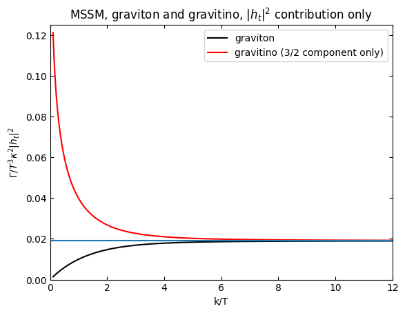
look at top Yukawa contribution and its UV asymptotics. At large \(k\gg T\) we have \(\frac{63 \zeta (3)}{128 \pi ^3}\approx 0.019\)
[7]:
gravitonrateplotht=graviton.rate(k,1,(0,0,0,1),0)
gravitinorateplothtdict=gravitino.rate(k,1,(0,0,0,1),0)
[59]:
plt.rcParams['ytick.right'] = True
plt.rcParams['ytick.labelright'] = False
plt.rcParams['ytick.left'] = plt.rcParams['ytick.labelleft'] = True
plt.rcParams["xtick.top"] =  True
plt.rcParams['xtick.direction']='in'
plt.rcParams['ytick.direction']='in'
plt.plot(k,gravitonrateplotht[1],"k",label="graviton")

plt.plot(k,gravitinorateplothtdict[1],"r",label="gravitino (3/2 component only)")

plt.xlim(0,12)
plt.ylim(0.,0.125)
#the UV limit is
from scipy.special import zeta

plt.axhline(63*zeta(3)/(128*numpy.pi**3))
plt.xlabel("k/T")
plt.ylabel(r"$\Gamma/T^3\kappa^2\vert h_t\vert^2$")
plt.title(r"MSSM, graviton and gravitino, $\vert h_t\vert^2$ contribution only")

plt.legend()
plt.show()
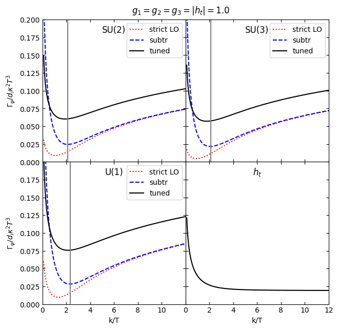
[89]:
fixcoupling=1.
couplings=[]
for i in range(4):
    coupvec=[0,0,0,0]
    coupvec[i]=fixcoupling
    couplings.append(coupvec)

plotres=[]
for coupling in couplings:
    temprate=gravitino.rate(k,1,(coupling),0)
    plotres.append(temprate)

plt.rcParams['ytick.right'] = True
plt.rcParams['ytick.labelright'] = False
plt.rcParams['ytick.left'] = plt.rcParams['ytick.labelleft'] = True
plt.rcParams["xtick.top"] =  True
plt.rcParams['xtick.direction']='in'
plt.rcParams['ytick.direction']='in'

fig=plt.figure()
cc=1.2
fig.set_size_inches(6*cc,6*cc)
gs = fig.add_gridspec(2, 2, hspace=0, wspace=0)
(ax, ax2) = gs.subplots(sharey='row',sharex='col')
myaxes=[ax[0],ax[1],ax2[0],ax2[1]]
labels=['SU(2)','SU(3)','U(1)',r'$h_t$']
mass=[numpy.sqrt(9/2)*fixcoupling,numpy.sqrt(9/2)*fixcoupling,numpy.sqrt(11/2)*fixcoupling,-1]
plotresshuffle=[plotres[1],plotres[2],plotres[0],plotres[3]]
norm=[1/3,1/8,1,1]
for i in range(4):
    myax=myaxes[i]
    if i<3:
        myax.plot(k,plotresshuffle[i][1]*norm[i],"r:",label='strict LO')
        myax.plot(k,plotresshuffle[i][2]*norm[i],"b--",label='subtr')
        myax.plot(k,plotresshuffle[i][3]*norm[i],"k",label="tuned")
        myax.legend()
    else:
         myax.plot(k,plotresshuffle[i][3]*norm[i],"k")
    myax.set_xlim(0,12)
    myax.axvline(mass[i],color='gray')
    if i==0:
        myax.set_ylim(0.,0.2)
        myax.set_ylabel(r'$\Gamma_\psi/d_i\kappa^2T^3$')
    if i==2:
        myax.set_ylim(0.,0.2)
        myax.set_ylabel(r'$\Gamma_\psi/d_i\kappa^2T^3$')
        myax.set_yticks(myax.get_yticks().tolist())
        myax.set_xticks(myax.get_xticks().tolist())
        tlabels = myax.get_yticklabels()
        # remove the last  label
        tlabels[-1] =  ""
        # set these new labels
        myax.set_yticklabels(tlabels)
        tlabels = myax.get_xticklabels()
        # remove the last  label
        tlabels[-1] =  ""
        # set these new labels
        myax.set_xticklabels(tlabels)
    if i>1:
        myax.set_xlabel('k/T')
    myax.set_title(labels[i],y=0.88)
# fig.supxlabel('k/T')
fig.suptitle(r'$g_1=g_2=g_3=|h_t|=$'+str(fixcoupling),y=0.92)
plt.savefig("../../../gravitinopaper/rate_"+str(fixcoupling)+".pdf",bbox_inches='tight')
plt.show()
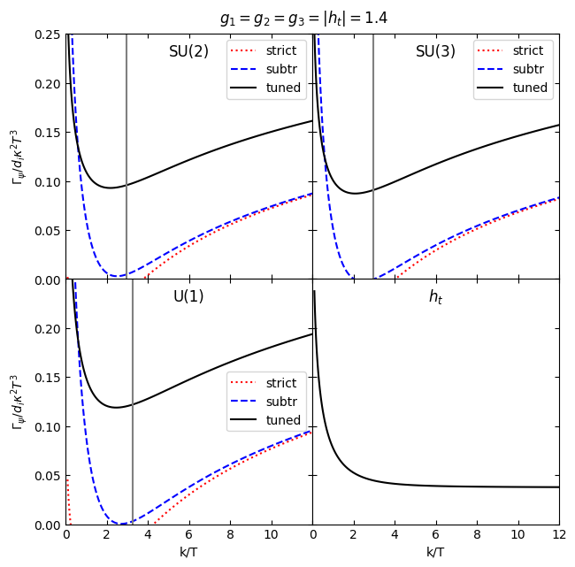
[90]:
fixcoupling=1.4
couplings=[]
for i in range(4):
    coupvec=[0,0,0,0]
    coupvec[i]=fixcoupling
    couplings.append(coupvec)

plotres=[]
for coupling in couplings:
    temprate=gravitino.rate(k,1,(coupling),0)
    plotres.append(temprate)

plt.rcParams['ytick.right'] = True
plt.rcParams['ytick.labelright'] = False
plt.rcParams['ytick.left'] = plt.rcParams['ytick.labelleft'] = True
plt.rcParams["xtick.top"] =  True
plt.rcParams['xtick.direction']='in'
plt.rcParams['ytick.direction']='in'

fig=plt.figure()
cc=1.2
fig.set_size_inches(6*cc,6*cc)
gs = fig.add_gridspec(2, 2, hspace=0, wspace=0)
(ax, ax2) = gs.subplots(sharey='row',sharex='col')
myaxes=[ax[0],ax[1],ax2[0],ax2[1]]
labels=['SU(2)','SU(3)','U(1)',r'$h_t$']
plotresshuffle=[plotres[1],plotres[2],plotres[0],plotres[3]]
mass=[numpy.sqrt(9/2)*fixcoupling,numpy.sqrt(9/2)*fixcoupling,numpy.sqrt(11/2)*fixcoupling,-1]

norm=[1/3,1/8,1,1]
for i in range(4):
    myax=myaxes[i]
    if i<3:
        myax.plot(k,plotresshuffle[i][1]*norm[i],"r:",label='strict')
        myax.plot(k,plotresshuffle[i][2]*norm[i],"b--",label='subtr')
        myax.plot(k,plotresshuffle[i][3]*norm[i],"k",label="tuned")
        myax.legend()
    else:
         myax.plot(k,plotresshuffle[i][3]*norm[i],"k")
    myax.set_xlim(0,12)
    myax.axvline(mass[i],color='gray')

    if i==0:
        myax.set_ylim(0.,0.25)
        myax.set_ylabel(r'$\Gamma_\psi/d_i\kappa^2T^3$')
    if i==2:
        myax.set_ylim(0.,0.25)
        myax.set_ylabel(r'$\Gamma_\psi/d_i\kappa^2T^3$')
        myax.set_yticks(myax.get_yticks().tolist())
        myax.set_xticks(myax.get_xticks().tolist())
        tlabels = myax.get_yticklabels()
        # remove the last  label
        tlabels[-1] =  ""
        # set these new labels
        myax.set_yticklabels(tlabels)
        tlabels = myax.get_xticklabels()
        # remove the last  label
        tlabels[-1] =  ""
        # set these new labels
        myax.set_xticklabels(tlabels)
    if i>1:
        myax.set_xlabel('k/T')
    myax.set_title(labels[i],y=0.88)
# fig.supxlabel('k/T')
fig.suptitle(r'$g_1=g_2=g_3=|h_t|=$'+str(fixcoupling),y=0.92)
plt.savefig("../../../gravitinopaper/rate_"+str(fixcoupling)+".pdf",bbox_inches='tight')
plt.show()
[91]:
fixcoupling=0.5
couplings=[]
for i in range(4):
    coupvec=[0,0,0,0]
    coupvec[i]=fixcoupling
    couplings.append(coupvec)

plotres=[]
for coupling in couplings:
    temprate=gravitino.rate(k,1,(coupling),0)
    plotres.append(temprate)

plt.rcParams['ytick.right'] = True
plt.rcParams['ytick.labelright'] = False
plt.rcParams['ytick.left'] = plt.rcParams['ytick.labelleft'] = True
plt.rcParams["xtick.top"] =  True
plt.rcParams['xtick.direction']='in'
plt.rcParams['ytick.direction']='in'

fig=plt.figure()
cc=1.2
fig.set_size_inches(6*cc,6*cc)
gs = fig.add_gridspec(2, 2, hspace=0, wspace=0)
(ax, ax2) = gs.subplots(sharey='row',sharex='col')
myaxes=[ax[0],ax[1],ax2[0],ax2[1]]
labels=['SU(2)','SU(3)','U(1)',r'$h_t$']
plotresshuffle=[plotres[1],plotres[2],plotres[0],plotres[3]]
mass=[numpy.sqrt(9/2)*fixcoupling,numpy.sqrt(9/2)*fixcoupling,numpy.sqrt(11/2)*fixcoupling,-1]
norm=[1/3,1/8,1,1]
for i in range(4):
    myax=myaxes[i]
    if i<3:
        myax.plot(k,plotresshuffle[i][1]*norm[i],"r:",label='strict')
        myax.plot(k,plotresshuffle[i][2]*norm[i],"b--",label='subtr')
        myax.plot(k,plotresshuffle[i][3]*norm[i],"k",label="tuned")
        myax.legend()
    else:
         myax.plot(k,plotresshuffle[i][3]*norm[i],"k")
    myax.set_xlim(0,12)
    myax.axvline(mass[i],color='gray')

    if i==0:
        myax.set_ylim(0.,0.06)
        myax.set_ylabel(r'$\Gamma_\psi/d_i\kappa^2T^3$')
    if i==2:
        myax.set_ylim(0.,0.06)
        myax.set_ylabel(r'$\Gamma_\psi/d_i\kappa^2T^3$')
        myax.set_yticks(myax.get_yticks().tolist())
        myax.set_xticks(myax.get_xticks().tolist())
        tlabels = myax.get_yticklabels()
        # remove the last  label
        tlabels[-1] =  ""
        # set these new labels
        myax.set_yticklabels(tlabels)
        tlabels = myax.get_xticklabels()
        # remove the last  label
        tlabels[-1] =  ""
        # set these new labels
        myax.set_xticklabels(tlabels)
    if i>1:
        myax.set_xlabel('k/T')
    myax.set_title(labels[i],y=0.88)
# fig.supxlabel('k/T')
fig.suptitle(r'$g_1=g_2=g_3=|h_t|=$'+str(fixcoupling),y=0.92)
plt.savefig("../../../gravitinopaper/rate_"+str(fixcoupling)+".pdf",bbox_inches='tight')

plt.show()
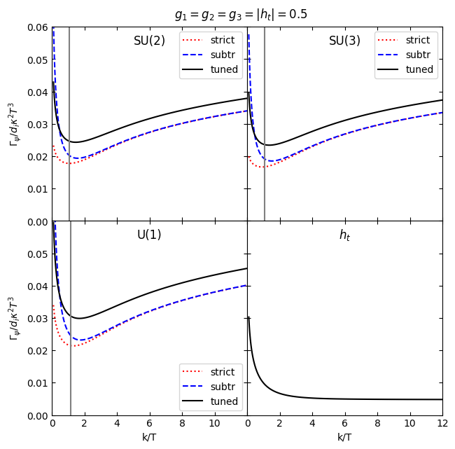
difference between SU(2) and SU(3) is the relatively larger Yukawa contribution wrt the (identical) gauge one for the former
do plots at a fixed temperature#
couplings from GUT, eq. (7) of 1512.05701 and (4.19) of Pradler’s master’s thesis. Weird that they would use \(T\) and not \(n\pi T\) as the scale
[5]:
def grun(T):
    beta=numpy.array([11,1,-3])
    mgut=2e16
    ggutsq=4*numpy.pi/24*numpy.array([3/5,1,1])
    gsq= ggutsq/(1-beta/(8*numpy.pi*numpy.pi)*ggutsq*numpy.log(T/mgut))
    #account for GUT U(1) normalisation
    return numpy.sqrt(gsq)

def grunpi(T):
    return grun(numpy.pi*T)
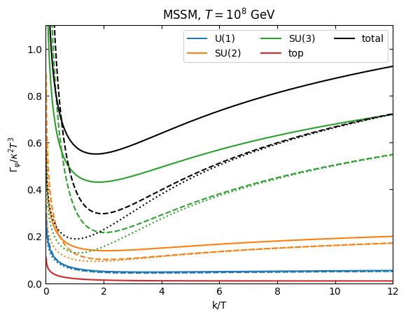
Do a plot at \(T=10^8\) GeV
[18]:
gaugecouplings=grunpi(1e8)
ht=0.7

kdense=numpy.linspace(0.01,15,1000)
gravitonrategauge=[]
gravitinorategauge=[]
for i in range(3):
    gaugevec = [0,0,0]
    gaugevec[i] = gaugecouplings[i]
    gravitonrategauge.append(graviton.rate(kdense,1,(*gaugevec,1),0))
    gravitinorategauge.append(gravitino.rate(kdense,1,(*gaugevec,1),0))

gravitonratetop=graviton.rate(kdense,1,(0,0,0,ht),0)
gravitinoratetop=gravitino.rate(kdense,1,(0,0,0,ht),0)

gravitonratetotal=graviton.rate(kdense,1,(*gaugecouplings,ht),0)
gravitinoratetotal=gravitino.rate(kdense,1,(*gaugecouplings,ht),0)
Warning raised by the integration routine for the dim-5 t-channel subtracted for momentum 11.72890890890891, statistics (1, 1, 1) and coefficients 1.
This is possibly not problematic. The warning message is:

The occurrence of roundoff error is detected, which prevents
  the requested tolerance from being achieved.  The error may be
  underestimated.
[ ]:
plt.rcParams['ytick.right'] = True
plt.rcParams['ytick.labelright'] = False
plt.rcParams['ytick.left'] = plt.rcParams['ytick.labelleft'] = True
plt.rcParams["xtick.top"] =  True
plt.rcParams['xtick.direction']='in'
plt.rcParams['ytick.direction']='in'
plt.plot(kdense,gravitinorategauge[0][1],"C0:")
plt.plot(kdense,gravitinorategauge[0][2],"C0--")
plt.plot(kdense,gravitinorategauge[0][3],"C0",label="U(1)")
plt.plot(kdense,gravitinorategauge[1][1],"C1:")
plt.plot(kdense,gravitinorategauge[1][2],"C1--")
plt.plot(kdense,gravitinorategauge[1][3],"C1",label="SU(2)")
plt.plot(kdense,gravitinorategauge[2][1],"C2:")
plt.plot(kdense,gravitinorategauge[2][2],"C2--")
plt.plot(kdense,gravitinorategauge[2][3],"C2",label="SU(3)")
plt.plot(kdense,gravitinoratetop[1],"C3",label='top')
plt.plot(kdense,gravitinoratetotal[1],"k:")
plt.plot(kdense,gravitinoratetotal[2],"k--")
plt.plot(kdense,gravitinoratetotal[3],"k",label="total")

plt.xlim(0,12)
plt.ylim(0,1.1)
plt.xlabel("k/T")
plt.ylabel(r"$\Gamma_\psi/\kappa^2T^3$")
plt.title(r"MSSM, $T=10^8$ GeV")

plt.legend(ncols=3)
plt.show()
[ ]:
plt.rcParams['ytick.right'] = True
plt.rcParams['ytick.labelright'] = False
plt.rcParams['ytick.left'] = plt.rcParams['ytick.labelleft'] = True
plt.rcParams["xtick.top"] =  True
plt.rcParams['xtick.direction']='in'
plt.rcParams['ytick.direction']='in'

fig,ax=plt.subplots()
fig.set_size_inches(3,3.5)

plt.plot(kdense,gravitinoratetotal[1],"C0",label=r"strict")
plt.plot(kdense,gravitonratetotal[1],"C0--")

plt.plot(kdense,gravitinoratetotal[2],"C1",label=r"subtr")
plt.plot(kdense,gravitonratetotal[2],"C1--")

plt.plot(kdense,gravitinoratetotal[3],"C2",label=r"tuned")
plt.plot(kdense,gravitonratetotal[3],"C2--")

plt.xlim(0,12.5)
plt.ylim(-0.1,1.)
plt.xlabel("k/T")
plt.ylabel(r"$\Gamma/\kappa^2T^3$")
plt.title(r"MSSM, $T=10^8$ GeV")
plt.axhline(0,color='k',linewidth=0.5)
plt.plot(kdense,10*gravitinoratetotal[3],"k",label=r"$\Gamma_\psi$")
plt.plot(kdense,10*gravitinoratetotal[3],"k--",label=r"$\Gamma_G$")

plt.legend(ncols=2)
plt.savefig('../../../gravitinopaper/susy_k.pdf',bbox_inches='tight')
plt.show()
[ ]:
plt.rcParams['ytick.right'] = True
plt.rcParams['ytick.labelright'] = False
plt.rcParams['ytick.left'] = plt.rcParams['ytick.labelleft'] = True
plt.rcParams["xtick.top"] =  True
plt.rcParams['xtick.direction']='in'
plt.rcParams['ytick.direction']='in'
phsp=kdense*kdense/(numpy.exp(kdense)+1.)/(2.*numpy.pi**2)
plt.plot(kdense,phsp*gravitinorategauge[0][1],"C0:")
plt.plot(kdense,phsp*gravitinorategauge[0][2],"C0--")
plt.plot(kdense,phsp*gravitinorategauge[0][3],"C0",label="U(1)")
plt.plot(kdense,phsp*gravitinorategauge[1][1],"C1:")
plt.plot(kdense,phsp*gravitinorategauge[1][2],"C1--")
plt.plot(kdense,phsp*gravitinorategauge[1][3],"C1",label="SU(2)")
plt.plot(kdense,phsp*gravitinorategauge[2][1],"C2:")
plt.plot(kdense,phsp*gravitinorategauge[2][2],"C2--")
plt.plot(kdense,phsp*gravitinorategauge[2][3],"C2",label="SU(3)")
plt.plot(kdense,phsp*gravitinoratetop[1],"C3",label='top')
plt.plot(kdense,phsp*gravitinoratetotal[1],"k:")
plt.plot(kdense,phsp*gravitinoratetotal[2],"k--")
plt.plot(kdense,phsp*gravitinoratetotal[3],"k",label="total")

plt.xlim(0,12)
plt.ylim(0,0.014)
plt.xlabel("k/T")
plt.ylabel(r"$\Gamma k^2 n_\mathrm{F}(k)/2\pi^2T^5\kappa^2$")
plt.title(r"MSSM $m_s=3/2$ gravitino rate, $T=10^8$ GeV")

plt.legend(ncols=3)
plt.show()

[ ]:
plt.rcParams['ytick.right'] = True
plt.rcParams['ytick.labelright'] = False
plt.rcParams['ytick.left'] = plt.rcParams['ytick.labelleft'] = True
plt.rcParams["xtick.top"] =  True
plt.rcParams['xtick.direction']='in'
plt.rcParams['ytick.direction']='in'

fig,(ax,ax2)=plt.subplots(ncols=2,figsize=(7,3.5))
fig.tight_layout(pad=3.2)

ax.plot(kdense,gravitinoratetotal[1],"C0",label=r"strict")
ax.plot(kdense,gravitonratetotal[1],"C0--")


ax.plot(kdense,gravitinoratetotal[2],"C1",label=r"subtr")
ax.plot(kdense,gravitonratetotal[2],"C1--")

ax.plot(kdense,gravitinoratetotal[3],"C2",label=r"tuned")
ax.plot(kdense,gravitonratetotal[3],"C2--")

ax.set_xlim(0,12.5)
ax.set_ylim(-0.1,1.)
ax.set_xlabel("k/T")
ax.set_ylabel(r"$\Gamma/\kappa^2T^3$")
ax.set_title(r"MSSM, $T=10^8$ GeV")
ax.axhline(0,color='k',linewidth=0.5)
ax.plot(kdense,10*gravitinoratetotal[3],"k",label=r"$\Gamma_\psi$")
ax.plot(kdense,10*gravitinoratetotal[3],"k--",label=r"$\Gamma_G$")

ax.legend(ncols=2)


phsp=kdense*kdense/(numpy.exp(kdense)+1.)#/(numpy.pi**2)
phspG=kdense*kdense/(numpy.expm1(kdense))#/(numpy.pi**2)
kdense2=numpy.insert(kdense,0,0.0001)
phspG2=kdense2*kdense2/(numpy.expm1(kdense2))#/(numpy.pi**2)
gravitonstrict= numpy.insert(gravitonratetotal[1],0,0.)


ax2.plot(kdense,phsp*gravitinoratetotal[1],"C0",label=r"strict")
ax2.plot(kdense2,phspG2*gravitonstrict,"C0--")

ax2.plot(kdense,phsp*gravitinoratetotal[2],"C1",label=r"subtr")
ax2.plot(kdense,phspG*gravitonratetotal[2],"C1--")

ax2.plot(kdense,phsp*gravitinoratetotal[3],"C2",label=r"tuned")
ax2.plot(kdense,phspG*gravitonratetotal[3],"C2--")

ax2.set_xlim(0,12.5)
ax2.set_ylim(-0.25,0.3)
ax2.set_xlabel("k/T")
ax2.set_ylabel(r"$\Gamma k^2 n(k)/T^5\kappa^2$")
ax2.set_title(r"MSSM, $T=10^8$ GeV")
ax2.axhline(0,color='k',linewidth=0.5)
ax2.plot(kdense,10*gravitinoratetotal[3],"k",label=r"$\Gamma_\psi$")
ax2.plot(kdense,10*gravitinoratetotal[3],"k--",label=r"$\Gamma_G$")

ax2.legend(ncols=2)
plt.savefig('../../../gravitinopaper/susy_combi.pdf',bbox_inches='tight')
plt.show()

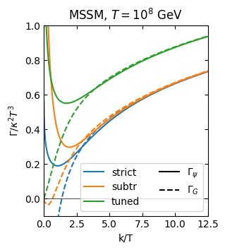
the figure above explains why negativity is much more dramatic in the axion case
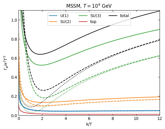
do the same plot at a lower temperature, 10 TeV
[24]:
gaugecouplingslow=grunpi(1e4)
ht=0.7

kdense2=numpy.logspace(-2,numpy.log10(12),100)
gravitonrategauge2=[]
gravitinorategauge2=[]
for i in range(3):
    gaugevec = [0,0,0]
    gaugevec[i] = gaugecouplingslow[i]
    gravitonrategauge2.append(graviton.rate(kdense2,1,(*gaugevec,1),0))
    gravitinorategauge2.append(gravitino.rate(kdense2,1,(*gaugevec,1),0))

gravitonratetop2=graviton.rate(kdense2,1,(0,0,0,ht),0)
gravitinoratetop2=gravitino.rate(kdense2,1,(0,0,0,ht),0)

gravitonratetotal2=graviton.rate(kdense2,1,(*gaugecouplingslow,ht),0)
gravitinoratetotal2=gravitino.rate(kdense2,1,(*gaugecouplingslow,ht),0)
[ ]:
plt.rcParams['ytick.right'] = True
plt.rcParams['ytick.labelright'] = False
plt.rcParams['ytick.left'] = plt.rcParams['ytick.labelleft'] = True
plt.rcParams["xtick.top"] =  True
plt.rcParams['xtick.direction']='in'
plt.rcParams['ytick.direction']='in'
plt.plot(kdense2,gravitinorategauge2[0][1],"C0:")
plt.plot(kdense2,gravitinorategauge2[0][2],"C0--")
plt.plot(kdense2,gravitinorategauge2[0][3],"C0",label="U(1)")
plt.plot(kdense2,gravitinorategauge2[1][1],"C1:")
plt.plot(kdense2,gravitinorategauge2[1][2],"C1--")
plt.plot(kdense2,gravitinorategauge2[1][3],"C1",label="SU(2)")
plt.plot(kdense2,gravitinorategauge2[2][1],"C2:")
plt.plot(kdense2,gravitinorategauge2[2][2],"C2--")
plt.plot(kdense2,gravitinorategauge2[2][3],"C2",label="SU(3)")
plt.plot(kdense2,gravitinoratetop2[1],"C3",label='top')
plt.plot(kdense2,gravitinoratetotal2[1],"k:")
plt.plot(kdense2,gravitinoratetotal2[2],"k--")
plt.plot(kdense2,gravitinoratetotal2[3],"k",label="total")

plt.xlim(0,12)
plt.ylim(0,1.1)
plt.xlabel("k/T")
plt.ylabel(r"$\Gamma_\psi/\kappa^2T^3$")
plt.title(r"MSSM, $T=10^4$ GeV")

plt.legend(ncols=3)
plt.show()
do the momentum integrands as in 2408.16043. The top one is constant, so we can treat it separately#
[ ]:
from scipy.integrate import trapezoid, quad, fixed_quad

# ngs=30
ngs=140
gvec=numpy.linspace(0.01,1.4,ngs)
# gvecG=numpy.linspace(0.01,1.4,ngs/4)
fnfinal=[]
fnfinalG=[]
for ik in range(0,ngs):
    print(ik,end="\r")
    fn=[[0,0,0],[0,0,0],[0,0,0]]
    fnG=[[0,0,0],[0,0,0],[0,0,0]]

    gtest=gvec[ik]
    def ratevec(x,j,i):
        #add factor of 2 for degeneracy
        #factor out factor of 1/pi^2
        statfac=x*x/(numpy.exp(x)+1.)
        coupvec=[0,0,0,0]
        coupvec[j]=gtest
        evalf=gravitino.rate(x,1,tuple(coupvec),i)[1]
        return statfac*evalf

    def ratevecG(x,j,i):
        #add factor of 2 for degeneracy
        #factor out factor of 1/pi^2
        statfac=x*x/(numpy.expm1(x))
        coupvec=[0,0,0,0]
        coupvec[j]=gtest
        evalf=graviton.rate(x,1,tuple(coupvec),i)[1]
        return statfac*evalf

    for j in range(0,3):
        for i in range(1,4):
            # fn[j][i-1]=quad(ratevec,0.,15.,args=(j,i),epsrel=1e-6)[0]/((gtest**2)*3*1.20206)*64*numpy.pi
            #fixed_quad with order n=20 is much faster than quad for the similar accuracy
            fn[j][i-1]=fixed_quad(ratevec,0.,15.,args=(j,i),n=20)[0]/((gtest**2)*3*1.20206)*64*numpy.pi
            # fnG[j][i-1]=quad(ratevecG,0.,15.,args=(j,i),epsrel=1e-6)[0]/((gtest**2)*4*1.20206)*64*numpy.pi
    fnfinal.append(fn)
    fnfinalG.append(fnG)
[ ]:
ngsG=30
# ngs=140
gvecG=numpy.linspace(0.01,1.4,ngsG)
# gvecG=numpy.linspace(0.01,1.4,ngs/4)
# fnfinal=[]
fnfinalG=[]
for ik in range(0,ngsG):
    print(ik,end="\r")
    # fn=[[0,0,0],[0,0,0],[0,0,0]]
    fnG=[[0,0,0],[0,0,0],[0,0,0]]

    gtest=gvecG[ik]

    def ratevecG(x,j,i):
        #add factor of 2 for degeneracy
        #factor out factor of 1/pi^2
        statfac=x*x/(numpy.expm1(x))
        coupvec=[0,0,0,0]
        coupvec[j]=gtest
        evalf=graviton.rate(x,1,tuple(coupvec),i)[1]
        return statfac*evalf

    for j in range(0,3):
        for i in range(1,4):
            # fn[j][i-1]=quad(ratevec,0.,15.,args=(j,i),epsrel=1e-6)[0]/((gtest**2)*3*1.20206)*64*numpy.pi
            # fnG[j][i-1]=quad(ratevecG,0.,15.,args=(j,i),epsrel=1e-6)[0]/((gtest**2)*4*1.20206)*64*numpy.pi
            fnG[j][i-1]=fixed_quad(ratevecG,0.,15.,args=(j,i),n=20)[0]/((gtest**2)*4*1.20206)*64*numpy.pi
    # fnfinal.append(fn)
    fnfinalG.append(fnG)
[78]:
numpy.save("../../../gravitinopaper/fnfinal.npy",fnfinal)
numpy.save("../../../gravitinopaper/fnfinalG.npy",fnfinalG)
[45]:
schemes=['strict','subtr','tuned']
for j,scheme in enumerate(schemes):
    filename = "../../../gravitinopaper/fi_"+scheme+".dat"
    file=open(filename,'w')
    file.write("# g_i\t\tF_1/(3 zeta(3))\t\tF_2/(3 zeta(3))\t\tF_3/(3 zeta(3))\n")
    for i in range(ngs):
        gsq=gvec[i]*gvec[i]
        file.write("%.2f\t\t%e\t\t%e\t\t%e\n"%(gvec[i],gsq*fnfinal[i][0][j],gsq*fnfinal[i][1][j]/3,gsq*fnfinal[i][2][j]/8))
    file.close()
The top contribution is in reasonable numerical agreeement with the value (1.30) given by Rychkov Strumia. 2408.16043 claims their matrix element squared is 12 times smaller, which would be problematic because it would break the SUSY relation between the graviton and the gravitino value. Keeping their (apparently more precise) numerical values, multiplying by 12 and accounting for normalisation, one finds
[30]:
0.25957*1e-3*6*12/9*2*numpy.pi**5
[30]:
1.2709364732754482
[30]:
mykdense=numpy.logspace(numpy.log10(0.01),numpy.log10(15),1000)
mykdense=numpy.linspace(0.01,15,1000)

ratetop=gravitino.rate(mykdense,1,(0.,0.,0.,1),0)
integrandtop=2*mykdense*mykdense*numpy.exp(-mykdense)/(numpy.exp(-mykdense)+1.)/(2*numpy.pi*numpy.pi)*ratetop[1]
trapezoid(integrandtop,mykdense)*8*numpy.pi**5/9
[30]:
so our result is kind of halfway between the two
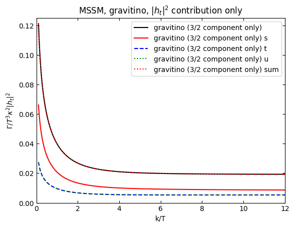
what happens if we treat separately the s, t and u Yukawa contributions?
[31]:
gravitinondictStop=({(-1,1,1):'kappa^2*ht^2*9*(s)'},{'gauge': (),'noneq': ('kappa',), 'others': ('ht',)},{})
gravitinotopS=NumRate(*gravitinondictStop,1)
gravitinondictTtop=({(1,1,-1):'-kappa^2*ht^2*9*(t)'},{'gauge': (),'noneq': ('kappa',), 'others': ('ht',)},{})
gravitinotopT=NumRate(*gravitinondictTtop,1)
gravitinondictUtop=({(1,-1,1):'-kappa^2*ht^2*9*(u)'},{'gauge': (),'noneq': ('kappa',), 'others': ('ht',)},{})
gravitinotopU=NumRate(*gravitinondictUtop,1)
[ ]:
gravitinorateplothtS=gravitinotopS.rate(k,1,(1,),0)
gravitinorateplothtT=gravitinotopT.rate(k,1,(1,),0)
gravitinorateplothtU=gravitinotopU.rate(k,1,(1,),0)
plt.rcParams['ytick.right'] = True
plt.rcParams['ytick.labelright'] = False
plt.rcParams['ytick.left'] = plt.rcParams['ytick.labelleft'] = True
plt.rcParams["xtick.top"] =  True
plt.rcParams['xtick.direction']='in'
plt.rcParams['ytick.direction']='in'

plt.plot(k,gravitinorateplothtdict[1],"k",label="gravitino (3/2 component only)")
plt.plot(k,gravitinorateplothtS[1],"r",label="gravitino (3/2 component only) s")
plt.plot(k,gravitinorateplothtT[1],"b--",label="gravitino (3/2 component only) t")
plt.plot(k,gravitinorateplothtU[1],"g:",label="gravitino (3/2 component only) u")
plt.plot(k,gravitinorateplothtS[1]+gravitinorateplothtT[1]+gravitinorateplothtU[1],"r:",label="gravitino (3/2 component only) sum")

plt.xlim(0,12)
plt.ylim(0.,0.125)
plt.xlabel("k/T")
plt.ylabel(r"$\Gamma/T^3\kappa^2\vert h_t\vert^2$")
plt.title(r"MSSM, gravitino, $\vert h_t\vert^2$ contribution only")

plt.legend()
plt.show()
[35]:
from scipy.integrate import quad
def integrand(x):
    return gravitinotopS.rate(x,1,(1,),0)[1]*x*x*numpy.exp(-x)/(numpy.exp(-x)+1.)

myres=quad(integrand,0.,numpy.inf)[0]*8*numpy.pi**3/9*2.
print(myres)
1.270918092424348
this is well within the numerical accuracy of the result provided by Eberl et al
[107]:
print("%.4e"%(myres/(6*12/9*2*numpy.pi**5)))
2.5957e-04
if we combine the s and t eberl result we get instead
[110]:
(6*12/9*2*numpy.pi**5)*(0.5*2.5957e-4+1.3286e-4)
[110]:
1.2859926417668837
[36]:
def integrand(x):
    return gravitinotopT.rate(x,1,(1,),0)[1]*x*x*numpy.exp(-x)/(numpy.exp(-x)+1.)

myresT=quad(integrand,0.,numpy.inf)[0]*8*numpy.pi**3/9*4.
print(myresT)
1.3010505839101127
[114]:
0.5*(myres+myresT)
[114]:
1.2859843381672302
[37]:
def integrand(x):
    return gravitino.rate(x,1,(0.,0.,0.,1),0)[1]*x*x*numpy.exp(-x)/(numpy.exp(-x)+1.)

myrestot=quad(integrand,0.,100.)[0]*8*numpy.pi**3/9
print(myrestot)
1.285984337290399
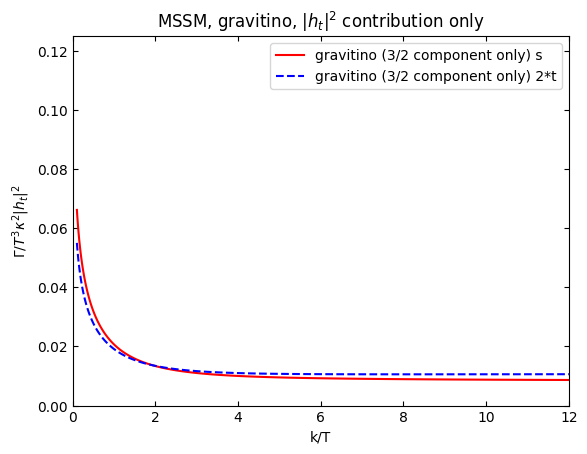
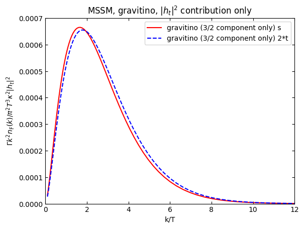
very suggestive: we get the Eberl result if we take twice the s-channel rate and we get the Rychkov result if we take twice the t+u rate.
[38]:
plt.plot(k,gravitinorateplothtS[1],"r",label="gravitino (3/2 component only) s")
plt.plot(k,2*gravitinorateplothtT[1],"b--",label="gravitino (3/2 component only) 2*t")
plt.xlim(0,12)
plt.ylim(0.,0.125)
plt.xlabel("k/T")
plt.ylabel(r"$\Gamma/T^3\kappa^2\vert h_t\vert^2$")
plt.title(r"MSSM, gravitino, $\vert h_t\vert^2$ contribution only")

plt.legend()
plt.show()

kfac=k*k/(numpy.exp(k)+1.)/(numpy.pi**2)

plt.plot(k,kfac*gravitinorateplothtS[1],"r",label="gravitino (3/2 component only) s")
plt.plot(k,kfac*2*gravitinorateplothtT[1],"b--",label="gravitino (3/2 component only) 2*t")
plt.xlim(0,12)
plt.ylim(0.,0.0007)
plt.xlabel("k/T")
plt.ylabel(r"$\Gamma k^2n_\mathrm{F}(k)/\pi^2T^3\kappa^2\vert h_t\vert^2$")
plt.title(r"MSSM, gravitino, $\vert h_t\vert^2$ contribution only")

plt.legend()
plt.show()
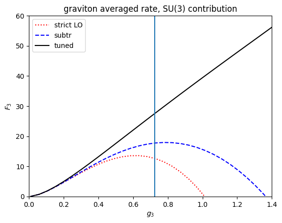
[30]:
qcdtuned=[]
qcdstrict=[]
qcdsubtr=[]
for line in fnfinal:
    qcdtuned.append(line[2][2])
    qcdstrict.append(line[2][0])
    qcdsubtr.append(line[2][1])
plt.plot(gvec,gvec**2*numpy.asarray(qcdstrict),"k:",label="strict LO")
plt.plot(gvec,gvec**2*numpy.asarray(qcdsubtr),"k--",label="subtr")
plt.plot(gvec,gvec**2*numpy.asarray(qcdtuned),"k",label="tuned")
plt.plot(gvec,2*20*gvec*gvec*numpy.log(3/gvec),"C0-.",label=r"1003.5847")
plt.plot(gvec,gvec**2*43.34 *numpy.log(3.041/gvec),"C1-.",label="1512.05701")
plt.plot(gvec,gvec**2*29.40 *numpy.log(3.07/gvec),"C2-.",label="2408.16043")

plt.plot(gvec,gvec**2*72 *numpy.log(1.271/gvec),"b:",label="hep-ph/0608344")


#put a vertical line at the value of the GUT coupling in 2408.16043. U(1) and SU(2) are only
#used at smaller couplings because of Landau pole, SU(3) at larger couplings because of asymptotic freedom
plt.axvline(numpy.sqrt(4*numpy.pi/24))
plt.title("averaged rate, SU(3) contribution")
plt.legend()
plt.xlim(0,1.4)
plt.ylim(0,80)
plt.xlabel(r"$g_3$")
plt.ylabel("$F_3$")

plt.show()


qcdtunedG=[]
qcdstrictG=[]
qcdsubtrG=[]
for line in fnfinalG:
    qcdtunedG.append(line[2][2])
    qcdstrictG.append(line[2][0])
    qcdsubtrG.append(line[2][1])
plt.plot(gvecG,gvecG**2*numpy.asarray(qcdstrictG),"r:",label="strict LO")
plt.plot(gvecG,gvecG**2*numpy.asarray(qcdsubtrG),"b--",label="subtr")
plt.plot(gvecG,gvecG**2*numpy.asarray(qcdtunedG),"k",label="tuned")
#put a vertical line at the value of the GUT coupling in 2408.16043. U(1) and SU(2) are only
#used at smaller couplings because of Landau pole, SU(3) at larger couplings because of asymptotic freedom
plt.axvline(numpy.sqrt(4*numpy.pi/24))
plt.title("graviton averaged rate, SU(3) contribution")
plt.legend()
plt.xlim(0,1.4)
plt.ylim(0,60)
plt.xlabel(r"$g_3$")
plt.ylabel("$F_3$")

plt.show()
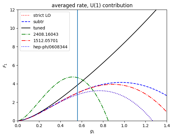
[31]:
u1tuned=[]
u1strict=[]
u1subtr=[]
for line in fnfinal:
    u1tuned.append(line[0][2])
    u1strict.append(line[0][0])
    u1subtr.append(line[0][1])
plt.plot(gvec,gvec**2*numpy.asarray(u1strict),"r:",label="strict LO")
plt.plot(gvec,gvec**2*numpy.asarray(u1subtr),"b--",label="subtr")
plt.plot(gvec,gvec**2*numpy.asarray(u1tuned),"k",label="tuned")
plt.plot(gvec,gvec**2*35.56 *numpy.log(0.85/gvec),"g-.",label="2408.16043")
# plt.plot(gvec,3/5*gvec**2*35.56 *numpy.log(0.85/gvec/numpy.sqrt(3/5)),"g-.",label="2408.16043")
plt.plot(gvec,gvec**2*9.90 *numpy.log(1.469/gvec),"r-.",label="1512.05701")
plt.plot(gvec,gvec**2*11 *numpy.log(1.266/gvec),"b:",label="hep-ph/0608344")

#put a vertical line at the value of the GUT coupling in 2408.16043. U(1) and SU(2) are only
#used at smaller couplings because of Landau pole, SU(3) at larger couplings because of asymptotic freedom
plt.axvline(numpy.sqrt(4*numpy.pi/24*3/5))
plt.ylim(0,12)
plt.xlim(0,1.4)
plt.title("averaged rate, U(1) contribution")
plt.legend()
plt.xlabel(r"$g_1$")
plt.ylabel("$F_1$")

plt.show()
[32]:
su2tuned=[]
su2strict=[]
su2subtr=[]
for line in fnfinal:
    su2tuned.append(line[1][2])
    su2strict.append(line[1][0])
    su2subtr.append(line[1][1])
plt.plot(gvec,gvec**2*numpy.asarray(su2strict),"r:",label="strict LO")
plt.plot(gvec,gvec**2*numpy.asarray(su2subtr),"b--",label="subtr")
plt.plot(gvec,gvec**2*numpy.asarray(su2tuned),"k",label="tuned")
plt.plot(gvec,gvec**2*35.33 *numpy.log(1.38/gvec),"g-.",label="2408.16043")
plt.plot(gvec,gvec**2*20.77 *numpy.log(2.071/gvec),"r-.",label="1512.05701")
# plt.plot(gvec,gvec**2*27 *numpy.log(1.312/gvec),"b:",label="hep-ph/0608344")
#put a vertical line at the value of the GUT coupling in 2408.16043. U(1) and SU(2) are only
#used at smaller couplings because of Landau pole, SU(3) at larger couplings because of asymptotic freedom
plt.axvline(numpy.sqrt(4*numpy.pi/24))
plt.title("averaged rate, SU(2) contribution")
plt.xlim(0,1.4)
plt.ylim(0,25)
plt.legend()
plt.xlabel(r"$g_2$")
plt.ylabel("$F_2$")
plt.show()
put these plots together
[18]:
plt.rcParams['ytick.right'] = True
plt.rcParams['ytick.labelright'] = False
plt.rcParams['ytick.left'] = plt.rcParams['ytick.labelleft'] = True
plt.rcParams["xtick.top"] =  True
plt.rcParams['xtick.direction']='in'
plt.rcParams['ytick.direction']='in'

fig=plt.figure()
cc=1.5
fig.set_size_inches(6*cc,2*cc)
gs = fig.add_gridspec(1, 3, hspace=0, wspace=0)
(ax, ax2,ax3) = gs.subplots(sharey=True)

#this is 3 \zeta(3) for the F_i normalisation
from scipy.special import zeta

zetanorm=3*zeta(3)
mdis=[11/2,9/2,9/2]
gnorm=[3/5,1,1]
aa=[ax,ax2,ax3]
styles=["k:","k--","k","C0-.","C1-."]
ax.plot(gvec,gvec**2*numpy.asarray(u1strict)*zetanorm,styles[0])
ax.plot(gvec,gvec**2*numpy.asarray(u1subtr)*zetanorm,styles[1])
ax.plot(gvec,gvec**2*numpy.asarray(u1tuned)*zetanorm,styles[2])
ax.plot(gvec,gvec**2*9.90 *numpy.log(1.469/gvec)*zetanorm,styles[3])
ax.plot(gvec,gvec**2*35.56 *numpy.log(0.85/gvec)*zetanorm,styles[4])
# plt.plot(gvec,gvec**2*11 *numpy.log(1.266/gvec),"b:",label="hep-ph/0608344")
#put a vertical line at the value of the GUT coupling in 2408.16043. U(1) and SU(2) are only
#used at smaller couplings because of Landau pole, SU(3) at larger couplings because of asymptotic freedom
ax.axvline(numpy.sqrt(4*numpy.pi/24*3/5),color='gray')
ax.set_ylim(0,40)
ax.set_xlim(0,1.4)
ax.set_title("U(1)")
# ax.legend()
ax.set_xlabel(r"$g_1$")
ax.set_ylabel("$F_i$")

su2norm=1/3*zetanorm
ax2.plot(gvec,gvec**2*numpy.asarray(su2strict)*su2norm,styles[0])
ax2.plot(gvec,gvec**2*numpy.asarray(su2subtr)*su2norm,styles[1])
ax2.plot(gvec,gvec**2*numpy.asarray(su2tuned)*su2norm,styles[2])
ax2.plot(gvec,gvec**2*20.77 *numpy.log(2.071/gvec)*su2norm,styles[3])
ax2.plot(gvec,gvec**2*35.33 *numpy.log(1.38/gvec)*su2norm,styles[4])
ax2.axvline(numpy.sqrt(4*numpy.pi/24),color='gray')
ax2.set_xlim(0,1.4)
ax2.set_xlabel(r"$g_2$")
ax2.set_title("SU(2)")

su3norm=1/8*zetanorm
ax3.plot(gvec,gvec**2*numpy.asarray(qcdstrict)*su3norm,styles[0],label="strict")
ax3.plot(gvec,gvec**2*numpy.asarray(qcdsubtr)*su3norm,styles[1],label="subtr")
ax3.plot(gvec,gvec**2*numpy.asarray(qcdtuned)*su3norm,styles[2],label="tuned")
ax3.plot(gvec,gvec**2*43.34 *numpy.log(3.041/gvec)*su3norm,styles[3],label="1512.05701")
ax3.plot(gvec,gvec**2*29.40 *numpy.log(3.07/gvec)*su3norm,styles[4],label="2408.16043")
ax3.plot(gvec,2*20*gvec*gvec*numpy.log(3/gvec)*su3norm,"C2-.",label=r"1003.5847")
ax3.axvline(numpy.sqrt(4*numpy.pi/24),color='gray')
ax3.set_xlim(0,1.4)
ax3.set_xlabel(r"$g_3$")
ax3.set_title("SU(3)")
plt.figlegend(loc='upper center',ncols=6,bbox_to_anchor=(0.5,1.1),bbox_transform=plt.gcf().transFigure)
plt.savefig("../../../gravitinopaper/fi.pdf",bbox_inches='tight')
plt.show()
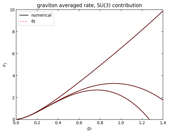
try some fits
[33]:
def fitf(g,a,b):
    return a*g*g*numpy.log(b/g)
def fitfN(g,a,b,c):
    return a*g*g*numpy.log(b/g)+c*g*g*g
from scipy.optimize import curve_fit
norm=1/8
poptstrict,pcovsstrict = curve_fit(fitfN,gvec,gvec*gvec*numpy.asarray(qcdstrict)*norm)
poptsubtr,pcovsubtr = curve_fit(fitfN,gvec,gvec*gvec*numpy.asarray(qcdsubtr)*norm)
popttuned,pcovtuned = curve_fit(fitfN,gvec,gvec*gvec*numpy.asarray(qcdtuned)*norm)
[34]:
plt.plot(gvec,gvec**2*numpy.asarray(qcdstrict)*norm,"k",label="numerical")
plt.plot(gvec,fitfN(gvec,*poptstrict),"r:",label="fit")


plt.plot(gvec,gvec**2*numpy.asarray(qcdsubtr)*norm,"k")
plt.plot(gvec,fitfN(gvec,*poptsubtr),"r:")


plt.plot(gvec,gvec**2*numpy.asarray(qcdtuned)*norm,"k")
plt.plot(gvec,fitfN(gvec,*popttuned),"r:")

#put a vertical line at the value of the GUT coupling in 2408.16043. U(1) and SU(2) are only
#used at smaller couplings because of Landau pole, SU(3) at larger couplings because of asymptotic freedom
# plt.axvline(numpy.sqrt(4*numpy.pi/24))
plt.title("gravitino averaged rate, SU(3) contribution")
plt.legend()
plt.xlim(0,1.4)
plt.ylim(0,80*norm)
plt.xlabel(r"$g_3$")
plt.ylabel("$F_3$")
plt.show()

[35]:
labels=['strict','subtr','tuned']
results=[poptstrict,poptsubtr,popttuned]
numresults=[qcdstrict,qcdsubtr,qcdtuned]
for i in range(3):
    myres=results[i]
    # if i==0:
        # myres=numpy.append(results[i],0.)
    print(labels[i]+"\ta=%.3f\tb=%.3f\tc=%.3f\tmax rel err=%.3e"%(myres[0],myres[1],myres[2],numpy.max(numpy.abs(1-fitfN(gvec,*results[i])/(gvec**2*numresults[i]*norm)))))
strict  a=9.000 b=1.271 c=-0.000        max rel err=3.339e-08
subtr   a=9.455 b=1.128 c=2.104 max rel err=2.520e-02
tuned   a=8.345 b=1.446 c=3.405 max rel err=4.794e-02
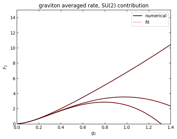
[36]:
norm=1/3
poptstrict,pcovsstrict = curve_fit(fitfN,gvec,gvec*gvec*numpy.asarray(su2strict)*norm)
poptsubtr,pcovsubtr = curve_fit(fitfN,gvec,gvec*gvec*numpy.asarray(su2subtr)*norm)
popttuned,pcovtuned = curve_fit(fitfN,gvec,gvec*gvec*numpy.asarray(su2tuned)*norm)
plt.plot(gvec,gvec**2*numpy.asarray(su2strict)*norm,"k",label="numerical")
plt.plot(gvec,fitfN(gvec,*poptstrict),"r:",label="fit")
# plt.plot(gvec,gvec**2*72 *numpy.log(1.271/gvec),"b-.",label="hep-ph/0608344")

plt.plot(gvec,gvec**2*numpy.asarray(su2subtr)*norm,"k")
plt.plot(gvec,fitfN(gvec,*poptsubtr),"r:")


plt.plot(gvec,gvec**2*numpy.asarray(su2tuned)*norm,"k")
plt.plot(gvec,fitfN(gvec,*popttuned),"r:")

#put a vertical line at the value of the GUT coupling in 2408.16043. U(1) and SU(2) are only
#used at smaller couplings because of Landau pole, SU(3) at larger couplings because of asymptotic freedom
# plt.axvline(numpy.sqrt(4*numpy.pi/24))
plt.title("gravitino averaged rate, SU(2) contribution")
plt.legend()
plt.xlim(0,1.4)
plt.ylim(0,15)
plt.xlabel(r"$g_2$")
plt.ylabel("$F_2$")
plt.show()
labels=['strict','subtr','tuned']
results=[poptstrict,poptsubtr,popttuned]
numresults=[su2strict,su2subtr,su2tuned]

for i in range(3):
    myres=results[i]
    # if i==0:
        # myres=numpy.append(results[i],0.)
    print(labels[i]+"\ta=%.3f\tb=%.3f\tc=%.3f\tmax rel err=%.3e"%(myres[0],myres[1],myres[2],numpy.max(numpy.abs(1-fitfN(gvec,*results[i])/(gvec**2*numresults[i]*norm)))))
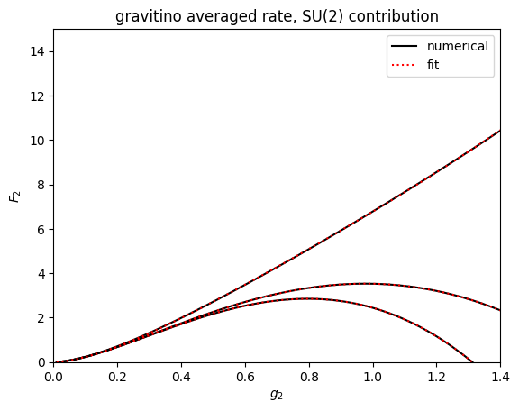
strict  a=9.000 b=1.312 c=0.000 max rel err=2.323e-08
subtr   a=9.455 b=1.163 c=2.104 max rel err=2.503e-02
tuned   a=8.345 b=1.497 c=3.405 max rel err=4.762e-02
[37]:
poptstrict,pcovsstrict = curve_fit(fitfN,gvec,gvec*gvec*numpy.asarray(u1strict))
poptsubtr,pcovsubtr = curve_fit(fitfN,gvec,gvec*gvec*numpy.asarray(u1subtr))
popttuned,pcovtuned = curve_fit(fitfN,gvec,gvec*gvec*numpy.asarray(u1tuned))
plt.plot(gvec,gvec**2*numpy.asarray(u1strict),"k",label="numerical")
plt.plot(gvec,fitfN(gvec,*poptstrict),"r:",label="fit")
# plt.plot(gvec,gvec**2*72 *numpy.log(1.271/gvec),"b-.",label="hep-ph/0608344")

plt.plot(gvec,gvec**2*numpy.asarray(u1subtr),"k")
plt.plot(gvec,fitfN(gvec,*poptsubtr),"r:")


plt.plot(gvec,gvec**2*numpy.asarray(u1tuned),"k")
plt.plot(gvec,fitfN(gvec,*popttuned),"r:")

#put a vertical line at the value of the GUT coupling in 2408.16043. U(1) and SU(2) are only
#used at smaller couplings because of Landau pole, SU(3) at larger couplings because of asymptotic freedom
# plt.axvline(numpy.sqrt(4*numpy.pi/24))
plt.title("gravitino averaged rate, U(1) contribution")
plt.legend()
plt.xlim(0,1.4)
plt.ylim(0,14)
plt.xlabel(r"$g_1$")
plt.ylabel("$F_1$")
plt.show()
labels=['strict','subtr','tuned']
results=[poptstrict,poptsubtr,popttuned]
numresults=[u1strict,u1subtr,u1tuned]
for i in range(3):
    myres=results[i]
    # if i==0:
        # myres=numpy.append(results[i],0.)
    print(labels[i]+"\ta=%.3f\tb=%.3f\tc=%.3f\tmax rel err=%.3e"%(myres[0],myres[1],myres[2],numpy.max(numpy.abs(1-fitfN(gvec,*results[i])/(gvec**2*numresults[i])))))
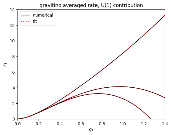
strict  a=10.999        b=1.266 c=-0.000        max rel err=2.896e-09
subtr   a=11.554        b=1.118 c=2.841 max rel err=2.406e-02
tuned   a=9.987 b=1.504 c=4.334 max rel err=5.982e-02
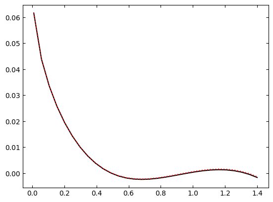
[88]:
plt.plot(gvec,1-fitfN(gvec,*popttuned)/gvec**2/u1tuned,"k")
plt.plot(gvec,1-fitfN(gvec,9.96,1.51,4.301)/gvec**2/u1tuned,"r:")
plt.show()

do an equivalent of fig. 12 of hep-ph/0701104
[ ]:
from scipy.integrate import quad_vec
def integrandvecvec(x,gvec):
    xfac = x*x*numpy.exp(-x)/(numpy.exp(-x)+1.)
    ratevec = [gravitino.rate(x,1,(gvec[0],0,0,0),0),gravitino.rate(x,1,(0,gvec[1],0,0),0),gravitino.rate(x,1,(0,0,gvec[2],0),0)]
    retvec=[]
    for j in range(0,3):
        for i in range(1,4):
            retvec.append(xfac*ratevec[j][i][0])
    return numpy.asarray(retvec).astype(numpy.float64)

ngs=30
Tvec=numpy.logspace(4,14,ngs)
fnfinalTquad=[]
for ik in range(0,ngs):
    print(ik,end="\r")
    fn=[[0,0,0],[0,0,0],[0,0,0]]

    gtest=grunpi(Tvec[ik])
    integral  = quad_vec(integrandvecvec,0.,20.,args=(gtest,))[0]
    for j in range(0,3):
        for i in range(1,4):

            fn[j][i-1]=4*integral[3*j+(i-1)]/numpy.pi**2
    fnfinalTquad.append(fn)
[51]:
mykdense=numpy.linspace(0.01,15,1000)

ratetop=gravitino.rate(mykdense,1,(0,0,0,1),0)
integrandtop=2*mykdense*mykdense*numpy.exp(-mykdense)/(numpy.exp(-mykdense)+1.)/(2*numpy.pi*numpy.pi)*ratetop[1]
toprate=trapezoid(integrandtop,mykdense)*4*numpy.ones(ngs)*ht**2
[ ]:
qcdtunedT=[]
qcdstrictT=[]
qcdsubtrT=[]
for line in fnfinalTquad:
    qcdtunedT.append(line[2][2])
    qcdstrictT.append(line[2][0])
    qcdsubtrT.append(line[2][1])
su2tunedT=[]
su2strictT=[]
su2subtrT=[]
for line in fnfinalTquad:
    su2tunedT.append(line[1][2])
    su2strictT.append(line[1][0])
    su2subtrT.append(line[1][1])
u1tunedT=[]
u1strictT=[]
u1subtrT=[]
for line in fnfinalTquad:
    u1tunedT.append(line[0][2])
    u1strictT.append(line[0][0])
    u1subtrT.append(line[0][1])

fig, ax= plt.subplots()
fig.set_size_inches(6,4.)
plt.plot(Tvec,numpy.asarray(qcdtunedT),"C2",label="SU(3)")

plt.plot(Tvec,numpy.asarray(qcdstrictT),"C2:")
plt.plot(Tvec,numpy.asarray(su2strictT),"C1:")

plt.plot(Tvec,numpy.asarray(su2tunedT),"C1",label="SU(2)")
plt.plot(Tvec,numpy.asarray(u1strictT),"C0:")

plt.plot(Tvec,numpy.asarray(u1tunedT),"C0",label="U(1)")
plt.plot(Tvec,toprate,"C3",label="top")


plt.plot(Tvec,numpy.asarray(u1tunedT)+numpy.asarray(su2tunedT)+numpy.asarray(qcdtunedT)+toprate,"k",label="total")
plt.plot(Tvec,numpy.asarray(u1strictT)+numpy.asarray(su2strictT)+numpy.asarray(qcdstrictT),"k:",label='strict LO')


plt.legend(ncols=3)
plt.xscale('log')
plt.xlim(1e4,1e14)
plt.ylim(0,0.6)
plt.xlabel(r"T/GeV")
plt.ylabel(r'$4\gamma_\psi/\kappa^2T^6$')

plt.minorticks_on()
plt.savefig('../../../gravitinopaper/gammaT.pdf',bbox_inches='tight')
plt.show()
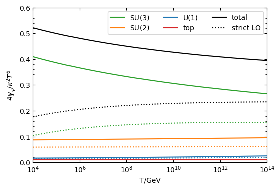
the total strict is in good agreement with the Pradler Steffen curve in fig 12 of rychkov strumia, as it should. If we subtract the top from it it should agree exactly
Axino production#
Define a running coupling as in (3.31) of hep-ph/0405158
[ ]:
def g3(T):
    return 1/numpy.sqrt(1/(4*numpy.pi*0.118)+3/(8*numpy.pi*numpy.pi)*numpy.log(T/91.19))
myg=g3(1e6)
import the dict (precomputed and stored in the json)
[ ]:
axinodict=analytical_pipeline("../../MyModels/mssm/mssm.cfg")
Configuration check completed successfully.
Skipping configuration.
Skipping generation of Feynman rules.
Skipping generation of all processes.
Analytical pipeline completed
pass the dict through the manipulate module and compute the rate
[ ]:
axino=NumRate(axinodict[0],axinodict[1],('(9*g3^2)/2',),1)
k=numpy.logspace(numpy.log10(0.1),numpy.log10(12.5),100)
axinorateplot=axino.rate(k,1,(myg,),0)
/var/folders/fd/k76vq6lj73v570m2x2k93yvm0000gp/T/ipykernel_59676/1359088618.py:1: AutothermWarning: Lack of direct proportionality between the gauge boson mass 9*g3**2/2 and the coefficient of the IR divergence -9*g3**6/(16*pi**4)
This is most likely not problematic, continuing with evaluation.
  axino=NumRate(axinodict[0],axinodict[1],('(9*g3^2)/2',),1)
[ ]:
axino.get_leadlog()
test this against the results that can be extracted from hep-ph/0405158
[ ]:
#axion dict from Steffen (rename kappa = 1/(32\pi^2  f_a/N)). Include factor of 2 to match normalisation
axinodictS = {(-1,-1,-1):"2*32*(1/(32*pi^2*  fpq))^2*g3^6*8*((s*u/t+t*u/s +s*t/u)*(3+nf))",\
              (1,1,-1):"2*32*(1/(32*pi^2  *fpq))^2*g3^6*8*((-t-2*s-2*s^2/t)*(3+nf)-3/2*t*nf)",\
               (-1,1,1): "2*16*(1/(32*pi^2 * fpq))^2*g3^6*8*((2*t^2/s)*(3+nf)+3/2*s*nf)"}
#note that the mass is different, the denominator is nc/2 and not 3 for the adjoint contribution,
# since we now have nc/3 from gluons and nc/6 from gluinos

axinotestS=NumRate(axinodictS, {"noneq":("fpq",),"gauge": ("g3",), "others": ("nf",)},\
                                ("g3^2*(3+nf)/2",),2)
axinorateplotS=axinotestS.rate(k,1,(myg,6.),0)
/var/folders/fd/k76vq6lj73v570m2x2k93yvm0000gp/T/ipykernel_59676/1233984401.py:8: AutothermWarning: Lack of direct proportionality between the gauge boson mass g3**2*nf/2 + 3*g3**2/2 and the coefficient of the IR divergence (-g3**6*nf - 3*g3**6)/(8*pi**4)
This is most likely not problematic, continuing with evaluation.
  axinotestS=NumRate(axinodictS, {"noneq":("fpq",),"gauge": ("g3",), "others": ("nf",)},\
[ ]:
plt.rcParams['ytick.right'] = True
plt.rcParams['ytick.labelright'] = False
plt.rcParams['ytick.left'] = plt.rcParams['ytick.labelleft'] = True
plt.rcParams["xtick.top"] =  True
plt.rcParams['xtick.direction']='in'
plt.rcParams['ytick.direction']='in'
plt.plot(k,axinorateplot[1],"g:",label="strict LO")
plt.plot(k,axinorateplotS[1],"k:",label="strict LO Steffen")
plt.plot(k,axinorateplot[2],"b--",label="subtracted")
plt.plot(k,axinorateplot[3],"r",label="tuned")
plt.xlim(0,12)
# plt.ylim(-0.00002,0.0001)
plt.xlabel("k/T")
plt.ylabel(r"$\Gamma_{a} f_\mathrm{PQ}^2/T^3$")
plt.title(r"axino, $T=10^6$ GeV")

plt.legend()
plt.show()
The discrepancy between the two “strict LO” results is due to the lack of the axino squark antisquark gluino coupling in hep-ph/0405158
do a plot of the F3 control function#
[ ]:
npoints=50
f3=[numpy.zeros(npoints),numpy.zeros(npoints),numpy.zeros(npoints)]
myk=numpy.logspace(numpy.log10(0.01),numpy.log10(15),100)
ivar = 0
myg3list = numpy.linspace(0.01,1.4,npoints)
for myg3 in myg3list:
    axinotemp = axino.rate(myk,1,(myg3,),0)
    for i in range(1,4):
        #add factor of 2 for degeneracy
        integrandaxinotest=2*myk*myk/(numpy.exp(myk)+1.)/(2*numpy.pi*numpy.pi)*axinotemp[i]
        f3[i-1][ivar]=trapezoid(integrandaxinotest,myk)/((myg3**4)/(256*(numpy.pi**7)))
    ivar=ivar+1
[ ]:
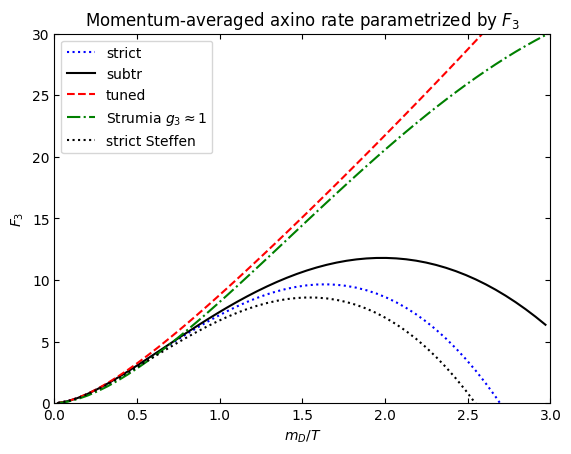
#add the asymptotitc behaviour from Eq. (9) in the Strumia axino paper
plt.plot(myg3list,f3[0],"b:",label="strict")
plt.plot(myg3list,f3[1],"k",label="subtr")
plt.plot(myg3list,f3[2],"r--",label="tuned")
plt.plot(myg3list,20*myg3list*myg3list*numpy.log(3/myg3list),"g-.",label=r"Strumia $g_3\approx 1$")
HTL=32.4*myg3list*myg3list*numpy.log(1.2/myg3list)
plt.plot(myg3list,HTL,"k:",label="strict Steffen")
plt.xlabel("$g_3$")
plt.ylabel("$F_3$")
plt.title("Momentum-averaged axino rate parametrized by $F_3$")
plt.legend()
plt.ylim(0,30)
plt.xlim(0,1.4)
plt.show()

[ ]:
#add the asymptotitc behaviour from Eq. (9) in the Strumia axino paper
plt.plot(myg3list*numpy.sqrt(9/2),f3[0],"b:",label="strict")
plt.plot(myg3list*numpy.sqrt(9/2),f3[1],"k",label="subtr")
plt.plot(myg3list*numpy.sqrt(9/2),f3[2],"r--",label="tuned")
plt.plot(myg3list*numpy.sqrt(9/2),20*myg3list*myg3list*numpy.log(3/myg3list),"g-.",label=r"Strumia $g_3\approx 1$")
HTL=32.4*myg3list*myg3list*numpy.log(1.2/myg3list)
plt.plot(myg3list*numpy.sqrt(9/2),HTL,"k:",label="strict Steffen")
plt.xlabel("$m_D/T$")
plt.ylabel("$F_3$")
plt.title("Momentum-averaged axino rate parametrized by $F_3$")
plt.legend()
plt.ylim(0,30)
plt.xlim(0,3)
plt.show()
[ ]:
#add the asymptotitc behaviour from Eq. (9) in the Strumia axino paper
plt.plot(myg3list*numpy.sqrt(9/4),f3[0],"b:",label="strict")
plt.plot(myg3list*numpy.sqrt(9/4),f3[1],"k",label="subtr")
plt.plot(myg3list*numpy.sqrt(9/4),f3[2],"r--",label="tuned")
plt.plot(myg3list*numpy.sqrt(9/4),20*myg3list*myg3list*numpy.log(3/myg3list),"g-.",label=r"Strumia $g_3\approx 1$")
HTL=32.4*myg3list*myg3list*numpy.log(1.2/myg3list)
plt.plot(myg3list*numpy.sqrt(9/4),HTL,"g:",label="strict Steffen")
plt.xlabel(r"$m_\infty/T$")
plt.ylabel("$F_3$")
plt.title("Momentum-averaged axino rate parametrized by $F_3$")
plt.legend()
plt.ylim(0,30)
plt.xlim(0,2.1)
plt.show()

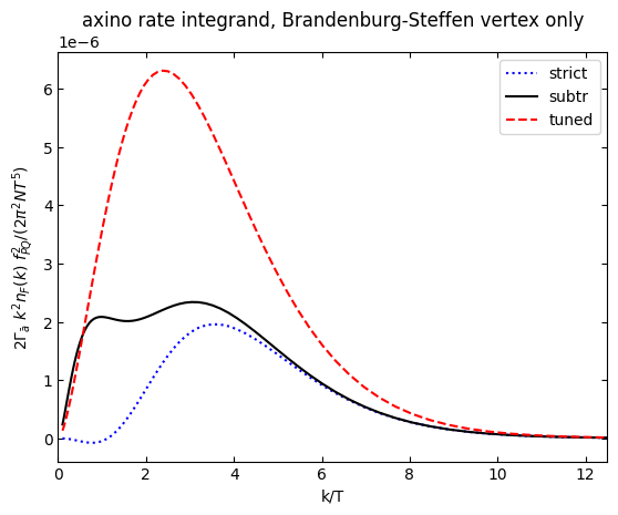
[ ]:
#create a numpy array for the integrand. add factor of 2 for the degeneracy
integrandaxinoS=[]
integrandaxino=[]
for i in range(1,4):
    integrandaxinoS.append(2*k*k/(numpy.exp(k)+1.)/(2*numpy.pi*numpy.pi)*axinorateplotS[i])
    integrandaxino.append(2*k*k/(numpy.exp(k)+1.)/(2*numpy.pi*numpy.pi)*axinorateplot[i])
plt.plot(k,integrandaxinoS[0],"b:",label="strict")
plt.plot(k,integrandaxinoS[1],"k",label="subtr")
plt.plot(k,integrandaxinoS[2],"r--",label="tuned")
plt.title(r"axino rate integrand, Brandenburg-Steffen vertex only")
plt.xlabel("k/T")
plt.ylabel(r"$2\Gamma_{\bar a}$ $k^2 n_F(k)$ $f_{PQ}^2$/($2\pi^2 N T^5$)")
plt.legend()
plt.xlim(0,12.5)
# plt.ylim(bottom=0)
plt.show()

[ ]:
plt.subplots(figsize=(6.75,5))
integralstrictS=trapezoid(integrandaxinoS[0],k)
integralsubtrS=trapezoid(integrandaxinoS[1],k)
integraltunedS=trapezoid(integrandaxinoS[2],k)
plt.plot(k,integrandaxinoS[0]/numpy.abs(integralstrictS),"b:",label="strict")
plt.plot(k,integrandaxinoS[1]/integralsubtrS,"k",label="subtr")
plt.plot(k,integrandaxinoS[2]/integraltunedS,"r--",label="tuned")

plt.title(r"axino rate integrand normalized by total integral, $T=10^6$ GeV, BS vertex only")
plt.xlabel("k/T")
plt.ylabel(r"$2\Gamma_{\bar a}$ $k^2 n_F(k)$ $f_{PQ}^2$/($2\pi^2 N T^5$ int)")
plt.legend()
plt.xlim(0,12.5)
plt.ylim(-0.1,0.3)
# plt.axis('off')

plt.show()
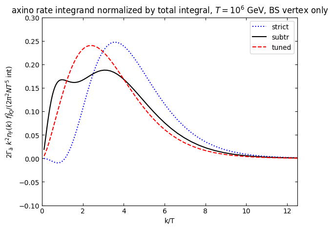
This is in good agreement with the figure in the erratum at the end of hep-ph/0405158
[ ]:
plt.subplots(figsize=(6.75,5))
integralstrictS=trapezoid(integrandaxinoS[0],k)
integralstrict=trapezoid(integrandaxino[0],k)
integralsubtr=trapezoid(integrandaxino[1],k)
integraltuned=trapezoid(integrandaxino[2],k)
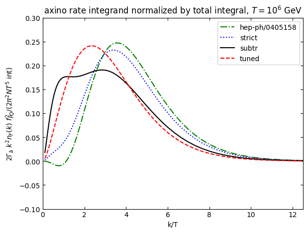
plt.plot(k,integrandaxinoS[0]/numpy.abs(integralstrictS),"g-.",label="hep-ph/0405158")
plt.plot(k,integrandaxino[0]/numpy.abs(integralstrict),"b:",label="strict")
plt.plot(k,integrandaxino[1]/integralsubtr,"k",label="subtr")
plt.plot(k,integrandaxino[2]/integraltuned,"r--",label="tuned")
plt.title(r"axino rate integrand normalized by total integral, $T=10^6$ GeV")
plt.xlabel("k/T")
plt.ylabel(r"$2\Gamma_{\bar a}$ $k^2 n_F(k)$ $f_{PQ}^2$/($2\pi^2 N T^5$ int)")
plt.legend()
plt.xlim(0,12.5)
plt.ylim(-0.1,0.3)
# plt.axis('off')
plt.show()