Dark Photon model, reproducing the results in 2212.09755

Importing the modules

#start by importing the controller and manipulate modules
from analytical.controller import *
from numerical.manipulate import *
#reimport numpy (though it is pulled by numerical) for smarter syntax highlighting in vscode
import numpy as np
#import matplotlib too
import matplotlib.pyplot as plt

Analytical part

The relevant part of the config file is as follows

[Model]
modelpath = /Users/jacopo/NextCloud/AUTOTHERM/autotherm/analytical/models/darkphoton.fr
# Symbol for the Lagrangian in the model file
lagrangian = Ltot
# "Name" of the particle whose production rate must be computed
produced = V[4]
# List of the particles in the thermal bath (or leave empty for SM assumption)
inbath =
assumptions = Element[M,Reals], Element[cb,Reals], Element[cbtilde,Reals],Element[cww,Reals], Element[cwwtilde,Reals],Element[cp,Reals], Element[cptilde,Reals], trcu>0, trcd>0, trce>0
replacements =
includeSM = yes
noneq = M
flavorexpand =

DP_analytical=analytical_pipeline("../../MyModels/darkphoton/darkphoton.cfg")

from IPython.display import display, Markdown
out=""
s = sympy.Symbol("s")
t = sympy.Symbol("t")
u = sympy.Symbol("u")
for key, item, in DP_analytical[0].items():
    sitem=sympy.sympify(item).subs(t+u,-s).subs(t*t+t*u,t*t+(s*s-t*t-u*u)/2).simplify()
    out+=f"- statistics: {key}: $${sympy.latex(sitem).replace('trcu',r'\mathrm{Tr}\,[C^\dagger_u C_u]')\
                                   .replace('trcd',r'\mathrm{Tr}\,[C^\dagger_d C_d]').replace('trce',r'\mathrm{Tr}\,[C^\dagger_e C_e]')\
                                    .replace('cb',r'c_b').replace('cww',r'c_w')}$$\n"
    # display(sympy.pprint(sitem))
display(Markdown(out))

• statistics: (1, -1, -1):

  \[\frac{64 t u \left(3 \mathrm{Tr}\,[C^\dagger_d C_d] + \mathrm{Tr}\,[C^\dagger_e C_e] + 3 \mathrm{Tr}\,[C^\dagger_u C_u]\right)}{M^{4}}\]

• statistics: (-1, -1, 1):

  \[- \frac{64 s u \left(3 \mathrm{Tr}\,[C^\dagger_d C_d] + \mathrm{Tr}\,[C^\dagger_e C_e] + 3 \mathrm{Tr}\,[C^\dagger_u C_u]\right)}{M^{4}}\]

• statistics: (-1, 1, -1):

  \[- \frac{64 s t \left(3 \mathrm{Tr}\,[C^\dagger_d C_d] + \mathrm{Tr}\,[C^\dagger_e C_e] + 3 \mathrm{Tr}\,[C^\dagger_u C_u]\right)}{M^{4}}\]

• statistics: (1, 1, 1):

  \[\frac{2 \left(s^{2} + t^{2} + u^{2}\right) \left(4 c_b^{2} + 4 \tilde{c_b}^{2} + 3 c_w^{2} + 3 \tilde{c_w}^{2}\right)}{M^{4}}\]

DP_analytical[1]

{'gauge': (),
 'noneq': ('M',),
 'others': ('cb', 'cbtilde', 'cww', 'cwwtilde', 'trcd', 'trce', 'trcu')}

compare this with the results of Salvio in 2212.09755.

(3.1) relates the rate (summed over polarisations) to the Wightman function.

(3.7) gives the sum over polarisations as \(16 K\cdot P(K\cdot P+Q\cdot P)\). If we look at fig. 1 and consider our (1,-1,-1) case (fermion fermion to boson boson) then \(K\cdot P=-t/2\) and \(Q\cdot P=-s/2\), so \(16 K\cdot P(K\cdot P+Q\cdot P)=-4 t(-t-s)=-4 t u\).

We thus expect for the (1,-1,-1) channel to find, including a factor of 2 to account for the \(1/(2P_0)\) normalisation (sum over the two polarisations), \(-8 C^2/M^4(-4 t u)=64 t u (3 \mathrm{Tr}\,[C^\dagger_u C_u]+3 \mathrm{Tr}\,[C^\dagger_d C_d] +\mathrm{Tr}\,[C^\dagger_e C_e])/M^4\). If we inspect the corresponding entry in DP_analytical[0] we find

display(Markdown(f"$${sympy.latex(sympy.sympify(DP_analytical[0][(1,-1,-1)])).replace('trcu',r'\mathrm{Tr}\,[C^\dagger_u C_u]')\
                                   .replace('trcd',r'\mathrm{Tr}\,[C^\dagger_d C_d]').replace('trce',r'\mathrm{Tr}\,[C^\dagger_e C_e]')\
                                    .replace('cb',r'c_b').replace('cww',r'c_w')}$$"))

\[\frac{64 t u \left(3 \mathrm{Tr}\,[C^\dagger_d C_d] + \mathrm{Tr}\,[C^\dagger_e C_e] + 3 \mathrm{Tr}\,[C^\dagger_u C_u]\right)}{M^{4}}\]

which agrees perfectly. The crossings obtained by moving a fermion to the final state are trivially checked too.

For the all-boson case we expect by applying the same logic to Eqs. (3.16) and (3.19) \(8\times 4/M^4 (c_b^2+\tilde{c}_b^2+c_w^2+\tilde{c}_{w}^2) (s^2/4+u^2/4+t^2/4)=16 (c_b^2+\tilde{c}_b^2+c_w^2+\tilde{c}_{w}^2) (t^2+u^2+ t u)/M^4\). We obtain

display(Markdown(f"$${sympy.latex(sympy.sympify(DP_analytical[0][(1,1,1)]).subs(t*t+t*u,t*t+(s*s-t*t-u*u)/2).simplify()).replace('trcu',r'\mathrm{Tr}\,[C^\dagger_u C_u]')\
                                   .replace('trcd',r'\mathrm{Tr}\,[C^\dagger_d C_d]').replace('trce',r'\mathrm{Tr}\,[C^\dagger_e C_e]')\
                                    .replace('cb',r'c_b').replace('cww',r'c_w')}$$"))

\[\frac{2 \left(s^{2} + t^{2} + u^{2}\right) \left(4 c_b^{2} + 4 \tilde{c_b}^{2} + 3 c_w^{2} + 3 \tilde{c_w}^{2}\right)}{M^{4}}\]

The abelian part (\(c_b\) and \(\tilde{c}_b\) coefficients) agrees with this. The non-abelian one does not: our result is a factor of 3/4 smaller, as it should, since 3/4 is the quadratic Casimir \((N^2-1)/(2N)\) for SU(\(N=2\)). Indeed, the Lagrangian in Eq. (2.1) should be intended, in its non-abelian part, as \(W^{\mu\nu}=W^{\mu\nu\,a} T^a\), with \(T^a\) the fundamental SU(2) generator, and likewise for \(\tilde{W}^{\mu\nu}\). When tracing over the SU(2) indices of the Higgs and \(W\) field in the squared amplitude, one finds indeed \((N^2-1)/(2N)\times N\) in the \(W\) case and $ N$ in the \(B\) case.

2212.09755 also notes that the diagram on the right in Fig. 2 vanishes. We remark that this is true in Feynman gauge but not necessarily in other gauges, as this diagram is just one of the many that contribute order-\(g_2^2\) corrections to the LO result. For instance, one of the two \(W\) bosons sourced by the non-abelian part of \(W^{\mu\nu}\) can attach to either of the Higgs lines. As our calculation is LO only, we do not consider this correction.

Numerical evaluation of the rate

DPB=NumRate(*DP_analytical,2)

/Users/jacopo/Nextcloud/AUTOTHERM/autotherm/.venv/lib/python3.12/site-packages/numerical/manipulate.py:428: AutothermWarning: Interaction of unsupported dimensionality, using C fallback mode
  temp = decompose(msq,stats,couplings)
/Users/jacopo/Nextcloud/AUTOTHERM/autotherm/.venv/lib/python3.12/site-packages/numerical/manipulate.py:428: AutothermWarning: Interaction of unsupported dimensionality, using C fallback mode
  temp = decompose(msq,stats,couplings)
/Users/jacopo/Nextcloud/AUTOTHERM/autotherm/.venv/lib/python3.12/site-packages/numerical/manipulate.py:428: AutothermWarning: Interaction of unsupported dimensionality, using C fallback mode
  temp = decompose(msq,stats,couplings)
/Users/jacopo/Nextcloud/AUTOTHERM/autotherm/.venv/lib/python3.12/site-packages/numerical/manipulate.py:428: AutothermWarning: Interaction of unsupported dimensionality, using C fallback mode
  temp = decompose(msq,stats,couplings)

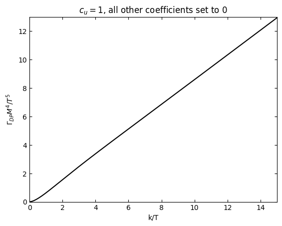
Look at the up-quark contribution, i.e. set trcu=1 and all other couplings to 0

k=numpy.logspace(numpy.log10(0.01),numpy.log10(15),300)
DPBrateup=DPB.rate(k,1,(0.,0.,0.,0.,0.,0.,1.),0)

plt.rcParams['ytick.right'] = True
plt.rcParams['ytick.labelright'] = False
plt.rcParams['ytick.left'] = plt.rcParams['ytick.labelleft'] = True
plt.rcParams["xtick.top"] =  True
plt.rcParams['xtick.direction']='in'
plt.rcParams['ytick.direction']='in'
plt.plot(k,DPBrateup[1],"k")

plt.xlim(0,15)
plt.ylim(0,13)
plt.xlabel("k/T")
plt.ylabel(r"$\Gamma_{DP} M^4/T^5$")
plt.title("$c_u=1$, all other coefficients set to 0")
# plt.legend()
plt.show()

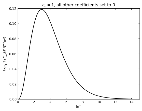
Look at the integrand corresponding to (3.3)

plt.rcParams['ytick.right'] = True
plt.rcParams['ytick.labelright'] = False
plt.rcParams['ytick.left'] = plt.rcParams['ytick.labelleft'] = True
plt.rcParams["xtick.top"] =  True
plt.rcParams['xtick.direction']='in'
plt.rcParams['ytick.direction']='in'
#multiply by 2k^2/(2\pi^2)n_B(k)
plt.plot(k,2*k*k/(2*numpy.pi**2)/np.expm1(k)*DPBrateup[1],"k")

plt.xlim(0,15)
plt.ylim(0,0.12)
plt.xlabel("k/T")
plt.ylabel(r"$k^2n_\mathrm{B}(k)\,\Gamma_{DP} M^4/(T^7\pi^2)$")
plt.title("$c_u=1$, all other coefficients set to 0")
# plt.legend()
plt.show()

Compute this integral

def fermiint(x):
    #factor out factor of 1/pi^2
    return DPB.rate(x,1,(0.,0.,0.,0.,0.,0.,1.),0)[1][0]*x*x/np.expm1(x)

from scipy.integrate import quad
print("%.6f"%(quad(fermiint,0,20.,epsrel=1e-6)[0]/np.pi/np.pi))

0.532767

(3.14) gives instead \(85.3 C^2 T^8/(\pi^6 M^4)\). This corresponds to \(85.3 \times 6 \,\mathrm{Tr}\,[C^\dagger_u C_u]\,T^8/(\pi^6 M^4)\), and

print("%.3f"%(85.3*6/np.pi**6))

0.532

which agrees with our numerical result. We can do the same for the all-boson processes, setting \(c_b\) to 1 and all other couplings to 0

def boseint(x):
    #factor out factor of 1/pi^2
    return DPB.rate(x,1,(1.,0.,0.,0.,0.,0.,0.),0)[1][0]*x*x/np.expm1(x)

from scipy.integrate import quad
print("%.6f"%(quad(boseint,0,20.,epsrel=1e-6)[0]/np.pi/np.pi))

0.042110

(3.18) gives instead \(40.5 (c_b^2+\tilde{c}_b^2) T^8/(\pi^6 M^4)\). Thus

print("%.3f"%(40.5/np.pi**6))

0.042

BETA: testing double production

We test the Higgs-Higgs going to DP DP contribution. We use our Mathematica package in autotherm.wl to compute this double-production process, i.e.

(* import packages *)
Get["~/Nextcloud/AUTOTHERM/FeynArts-3.12/FeynArts.m"];
Get["~/Nextcloud/AUTOTHERM/FormCalc-9.10/FormCalc.m"];
Get["~/Nextcloud/AUTOTHERM/FormCalc-9.10/tools/VecSet.m"];
Get["~/Nextcloud/AUTOTHERM/autotherm/analytical/autotherm.wl"]
(* load the config file for this model *)
ConfigParse["~/Nextcloud/AUTOTHERM/autotherm/MyModels/darkphoton/darkphoton.m"]
(* compute the matrix element squared *)
ComputeMatrixElement[{S[1], -S[1]} -> {V[4], V[4]}]

which returns

(16 S^2 AUTstatspart(1,1,1) (cp^2+cptilde^2))/M^4

We now create a dict for the manipulate module, adding a factor of two for swapping initial state particles, i.e. \(\bar\phi\phi\to\mathcal{P}\mathcal{P}\). We then exploit a feature of this module, namely that setting the statistics of the first outgoing particle to 0 enables us to consider double production by dropping the corresponding final state factor. We also set the degeneracy to 4, since 4 DP states are produced.

doublemsqdict={(0,1,1):'(32*(cp^2 + cptilde^2)*s^2)/M^4'}
couplingdict={'gauge':(),'noneq':('M',),'others':('cp','cptilde')}
dp=NumRate(doublemsqdict,couplingdict,(),4)

/Users/jacopo/Nextcloud/AUTOTHERM/autotherm/.venv/lib/python3.12/site-packages/numerical/manipulate.py:428: AutothermWarning: Interaction of unsupported dimensionality, using C fallback mode
  temp = decompose(msq,stats,couplings)

double=dp.rate(k,1,(1,1),0)[1]

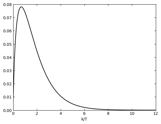
what comes out is minus the rate multiplied by the statistical function of particle 4, i.e. the production rate. This happens because the factorisation identities we use for n(s1,p1)n(s2,p2)(1+n(t1,k1))/n(t2,k) work differently if t1=0 than if |t1|=1.

plt.plot(k,-double,"k")

plt.xlim(0,12)
plt.ylim(0,0.08)
plt.xlabel("k/T")
# plt.ylabel(r"$\Gamma_{DP} M^4/T^5$")
# plt.title("$c_u=1$, all other coefficients set to 0")
# plt.legend()
plt.show()

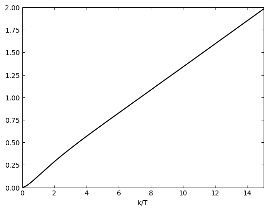
Hence, if we divide by the statistical function we get an analogue of the interaction rate

plt.plot(k,-double*numpy.expm1(k),"k")

plt.xlim(0,15)
plt.ylim(0,2)
plt.xlabel("k/T")
# plt.ylabel(r"$\Gamma_{DP} M^4/T^5$")
# plt.title("$c_u=1$, all other coefficients set to 0")
# plt.legend()
plt.show()

do the total integration. We include a factor of 4 for the two spin degrees of freedom and compare with (3.25) and (3.26) in Salvio. The factor of 2 at the denominator arises from our having set \(c_p\) and \(\tilde{c}_p\) to 1. Our result is a factor of 2 larger.

def doubleint(x):
    #factor out factor of 1/pi^2
    return -dp.rate(x,1,(1.,1.),0)[1][0]*x*x
print("%.6f"%(quad(doubleint,0.,20.,epsrel=1e-6)[0]*675*2/(2*numpy.pi**5)))

1.999995

The disagreement could be explained by a lack of a factor of 2 between (3.21) and (3.23) to account for the complex nature of the Higgs doublet and thus of the distinct \(\bar\phi\phi\) and \(\phi\bar\phi\) initial states.