Ultrarelativistic right-handed neutrino production, reproducing the \(2\leftrightarrow 2\) part of 1202.1288#
Importing the modules#
[1]:
#start by importing the controller and manipulate modules
from analytical.controller import *
from numerical.manipulate import *
#reimport numpy (though it is pulled by numerical) for smarter syntax highlighting in vscode
import numpy
#import matplotlib too
import matplotlib.pyplot as plt
Field-theoretical component#
The relevant part of the config file is as follows
[Model]
modelpath = /Users/jacopo/NextCloud/AUTOTHERM/autotherm/analytical/models/rhn.fr
# Symbol for the Lagrangian in the model file
lagrangian = Ltot
# "Name" of the particle whose production rate must be computed
produced = F[6]
# List of the particles in the thermal bath (or leave empty for SM assumption)
inbath =
assumptions = Element[hhh,Reals]
replacements =
includeSM = yes
noneq = hhh
#comma-separated list of particles to be treated with a flavor expansion
flavorexpand =
[ ]:
rhn_analytical=analytical_pipeline("../../MyModels/RHN/RHN.cfg")
Inspect the output. The hhh coupling in the model file stands for \(\sqrt{\mathrm{Tr}h^\dagger h}\), with \(h\) the Yukawa matrix between the right-handed neutrinos and the left-handed lepton doublet. In this models there are three generations of massless right-handed neutrinos.
[3]:
from IPython.display import display, Markdown
out=""
s = sympy.Symbol("s")
t = sympy.Symbol("t")
u = sympy.Symbol("u")
g1 = sympy.Symbol("g1")
g2 = sympy.Symbol("g2")
g3 = sympy.Symbol("g3")
ht = sympy.Symbol("ht")
hhh=sympy.Symbol("hhh")
for key, item, in rhn_analytical[0].items():
    sitem=sympy.simplify(sympy.sympify(item).subs(2*t*u,(s*s-t*t-u*u)))
    sitemsubst= sitem
    if sitemsubst.as_coeff_Add()[0] ==0:
        sitemsubstcollect = sitemsubst
    else:
        sitemsubstcollect=0
        for exprtemp in sympy.factor(sitemsubst.expand().as_independent(ht)).subs(t+u,-s)\
            .subs(2*t*t+2*t*u,2*t*t+(s*s-t*t-u*u)).subs(t*t+2*t*u,t*t+(s*s-t*t-u*u)).subs(t*t+t*u,t*t+(s*s-t*t-u*u)/2):
            sitemsubstcollect += exprtemp.simplify()
        # beautify the output
    out+=f"-  $$ \\left\\vert \\mathcal{{M}}({key[0]};{key[1]},{key[2]})\\right\\vert^2={sympy.latex(sitemsubstcollect).replace('ht^{2}',r'\vert h_t\vert^2').\
                                    replace('hhh^{2}',r'\mathrm{Tr}[h^\dagger h]')}$$\n"
    # display(sympy.pprint(sitem))
display(Markdown(out))
- \[\left\vert \mathcal{M}(-1;-1,-1)\right\vert^2=36 \mathrm{Tr}[h^\dagger h] \vert h_t\vert^2\]
- \[\left\vert \mathcal{M}(1;-1,1)\right\vert^2=- \frac{\mathrm{Tr}[h^\dagger h] \left(g_{1}^{2} + 3 g_{2}^{2}\right) \left(s^{2} + t^{2}\right)}{s t}\]
- \[\left\vert \mathcal{M}(1;1,-1)\right\vert^2=- \frac{\mathrm{Tr}[h^\dagger h] \left(g_{1}^{2} + 3 g_{2}^{2}\right) \left(s^{2} + u^{2}\right)}{s u}\]
- \[\left\vert \mathcal{M}(-1;1,1)\right\vert^2=\frac{\mathrm{Tr}[h^\dagger h] \left(g_{1}^{2} + 3 g_{2}^{2}\right) \left(t^{2} + u^{2}\right)}{t u}\]
Numerical part#
First, we must call NumRate#
We set the degeneracy to unity, since we are treating the right-handed neutrinos as massless and thus distinct from their antiparticles. The rate for the latter is then equal to that for the former that is determined here
[4]:
rate_rhn=NumRate(*rhn_analytical,1)
The leading-log term reads
[5]:
leadlog=rate_rhn.get_leadlog().simplify()
leadlog
[5]:
reexpress this in terms of the lepton asymptotic mass
[6]:
minf = sympy.Symbol(r"m_{\infty\,L}^2")
htrace=sympy.Symbol(r'\mathrm{Tr}[h^\dagger h]')
T = sympy.S("T")
k= sympy.S("k")
nB= sympy.Function("n_B")
leadlog.subs(g2*g2,16*(minf/T/T-g1*g1/16)/3).subs(sympy.tanh(k/(2*T)),1/(1+2* nB(k))).subs(hhh*hhh,htrace).simplify()
[6]:
This agrees with Eqs. (24) and (28) of of 1202.1288 and with (4.23) of 1605.07720
Now prepare to compare with the integration results in (29) of of 1202.1288
[7]:
#prepare to compute the total rate in the strict LO scheme
def ratevec(x,g1,g2,ht):
    #add factor of 2 for the "antiparticle"
    #factor out factor of 2/(2\pi^2)
    statfac=x*x/(numpy.exp(x)+1.)
    evalf=rate_rhn.rate(x,1,tuple([g1,g2,ht]),1)[1][0]
    return statfac*evalf
we first test \(c_Q\)
[8]:
from scipy.integrate import quad
#re-instate factor of 2/(2\pi^2)
yukawaint=1/numpy.pi**2*quad(ratevec,0.,20.,args=(1e-7,1e-7,1),epsrel=1e-5)[0]
display(Markdown(r'### We find $c_Q$=%.5f'%(yukawaint*1536*numpy.pi)))
We find \(c_Q\)=2.52136#
It checks out! Let us then test \(c_V\)
[10]:
g1test=1
g2test=1
gaugeint=1/numpy.pi**2*quad(ratevec,0.,20.,args=(g1test,g2test,0.),epsrel=1e-5)[0]
display(Markdown(r'### We find $c_V$=%.5f'%(gaugeint*1536*numpy.pi/(g1test**2+3*g2test**2)+numpy.log(g1test**2+3*g2test**2))))
We find \(c_V\)=3.16693#
Checks out as well!
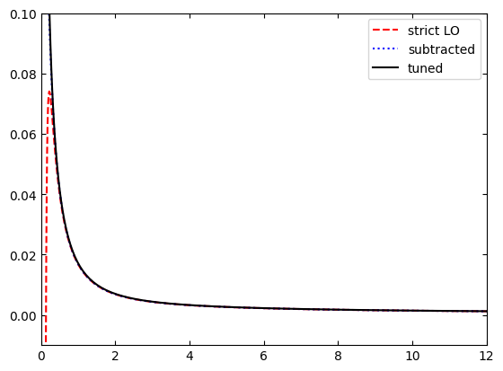
Plot the rate at \(T=200\) GeV. Couplings chosen along the procedure of 2004.11392#
[ ]:
k=numpy.geomspace(0.01,15,100)
coups=(numpy.sqrt(0.13031),numpy.sqrt(0.406827),numpy.sqrt(0.718285))
rateplt=rate_rhn.rate(k,1,coups,0)
[21]:
styles=["r--","b:","k"]
labels = ["strict LO","subtracted","tuned"]

plt.rcParams['ytick.right'] = True
plt.rcParams['ytick.labelright'] = False
plt.rcParams['ytick.left'] = plt.rcParams['ytick.labelleft'] = True
plt.rcParams["xtick.top"] =  True
plt.rcParams['xtick.direction']='in'
plt.rcParams['ytick.direction']='in'

plt.plot(k,rateplt[1],styles[0],label=labels[0])
plt.plot(k,rateplt[2],styles[1],label=labels[1])
plt.plot(k,rateplt[3],styles[2],label=labels[2])
plt.legend()
plt.xlim(0.,12.)
plt.ylim(-0.01,0.1)
plt.show()
[ ]: