Hot axion production, reproducing 2404.06113#
Importing the modules#
[1]:
#start by importing the controller and manipulate modules
from analytical.controller import *
from numerical.manipulate import *
#reimport numpy (though it is pulled by numerical) for smarter syntax highlighting in vscode
import numpy
#import matplotlib too
import matplotlib.pyplot as plt
Field-theoretical component#
The relevant part of the config file is as follows
[Model]
modelpath = /Users/jacopo/NextCloud/AUTOTHERM/autotherm/analytical/models/axion.fr
# Symbol for the Lagrangian in the model file
lagrangian = Ltot
# "Name" of the particle whose production rate must be computed
produced = S[2]
# List of the particles in the thermal bath (or leave empty for SM assumption)
inbath =
assumptions = Element[ht,Reals], Element[c1,Reals],Element[c2,Reals],Element[c3,Reals], Element[ct,Reals],Element[fPQ,Reals]
replacements =
includeSM = yes
noneq = fPQ
#comma-separated list of particles to be treated with a flavor expansion
flavorexpand =
[ ]:
axion_dict=analytical_pipeline("../../MyModels/axion/axion.cfg")
Let us look at this in detail. We have used the most generic axion-SM Lagrangian, with four Wilson coefficients for couplings to the gauge bosons and the top quark
[3]:
from IPython.display import display, Markdown
out=""
s = sympy.Symbol("s")
t = sympy.Symbol("t")
u = sympy.Symbol("u")
for key, item, in axion_dict[0].items():
    sitem=sympy.simplify(sympy.sympify(item).subs(2*t*t+2*t*u,2*t*t+(s*s-t*t-u*u)).subs(t*t+2*t*u,t*t+(s*s-t*t-u*u)).subs(t*t+t*u,t*t+(s*s-t*t-u*u)/2))
    out+=f"-  $$ \\left\\vert \\mathcal{{M}}({key[0]};{key[1]},{key[2]})\\right\\vert^2={sympy.latex(sitem).replace('ht^{2}',r'\vert h_t\vert^2').replace('fPQ^{2}',r'f_\mathrm{PQ}^2')}$$\n"
    # display(sympy.pprint(sitem))
display(Markdown(out))
- \[\left\vert \mathcal{M}(1;-1,-1)\right\vert^2=\frac{768 \pi^{4} ct^{2} \vert h_t\vert^2 s^{2} + \left(t^{2} + u^{2}\right) \left(5 c_{1}^{2} g_{1}^{6} + 9 c_{2}^{2} g_{2}^{6} + 24 c_{3}^{2} g_{3}^{6}\right)}{32 \pi^{4} f_\mathrm{PQ}^2 s}\]
- \[\left\vert \mathcal{M}(-1;-1,1)\right\vert^2=- \frac{5 c_{1}^{2} g_{1}^{6} \left(s^{2} + u^{2}\right) + 9 c_{2}^{2} g_{2}^{6} \left(s^{2} + u^{2}\right) + 24 c_{3}^{2} g_{3}^{6} \left(s^{2} + u^{2}\right) + 768 \pi^{4} ct^{2} \vert h_t\vert^2 t^{2}}{32 \pi^{4} f_\mathrm{PQ}^2 t}\]
- \[\left\vert \mathcal{M}(-1;1,-1)\right\vert^2=- \frac{5 c_{1}^{2} g_{1}^{6} \left(s^{2} + t^{2}\right) + 9 c_{2}^{2} g_{2}^{6} \left(s^{2} + t^{2}\right) + 24 c_{3}^{2} g_{3}^{6} \left(s^{2} + t^{2}\right) + 768 \pi^{4} ct^{2} \vert h_t\vert^2 u^{2}}{32 \pi^{4} f_\mathrm{PQ}^2 u}\]
- \[\left\vert \mathcal{M}(1;1,1)\right\vert^2=\frac{\left(s^{2} + t^{2} + u^{2}\right)^{2} \left(c_{1}^{2} g_{1}^{6} + 15 c_{2}^{2} g_{2}^{6} + 48 c_{3}^{2} g_{3}^{6}\right)}{256 \pi^{4} f_\mathrm{PQ}^2 s t u}\]
If we just want the KSVZ model, we can set \(c_3=1\) and all others to zero. We can also set the number of light quarks \(N_f\) as a dynamical degree of freedom
[4]:
out=""
s = sympy.Symbol("s")
t = sympy.Symbol("t")
u = sympy.Symbol("u")
nf = sympy.Symbol("nf")
ksvz_dict_msq={}
for key, item, in axion_dict[0].items():
    sitem=sympy.simplify(sympy.sympify(item).subs(2*t*t+2*t*u,2*t*t+(s*s-t*t-u*u)).subs(t*t+2*t*u,t*t+(s*s-t*t-u*u)).subs(t*t+t*u,t*t+(s*s-t*t-u*u)/2)\
        .subs(sympy.S('c3'),1).subs(sympy.S('c2'),0).subs(sympy.S('c1'),0).subs(sympy.S('ct'),0))
    if key[0]==-1 or key[1]==-1 or key[2]==-1:
        sitem = sitem*nf/6
    out+=f"-  $$ \\left\\vert \\mathcal{{M}}({key[0]};{key[1]},{key[2]})\\right\\vert^2={sympy.latex(sitem).replace('fPQ^{2}',r'f_\mathrm{PQ}^2').replace('nf',r'N_f')}$$\n"
    ksvz_dict_msq[key]=str(sitem)
    # display(sympy.pprint(sitem))
ksvz_dict_coups={'gauge':('g3',),'noneq':('fPQ',),'others':('nf',)}
ksvz_masses=('g3**2*(1+nf/6)',)
ksvz_dict=[ksvz_dict_msq,ksvz_dict_coups,ksvz_masses]
display(Markdown(out))
- \[\left\vert \mathcal{M}(1;-1,-1)\right\vert^2=\frac{g_{3}^{6} N_f \left(t^{2} + u^{2}\right)}{8 \pi^{4} f_\mathrm{PQ}^2 s}\]
- \[\left\vert \mathcal{M}(-1;-1,1)\right\vert^2=\frac{g_{3}^{6} N_f \left(- s^{2} - u^{2}\right)}{8 \pi^{4} f_\mathrm{PQ}^2 t}\]
- \[\left\vert \mathcal{M}(-1;1,-1)\right\vert^2=\frac{g_{3}^{6} N_f \left(- s^{2} - t^{2}\right)}{8 \pi^{4} f_\mathrm{PQ}^2 u}\]
- \[\left\vert \mathcal{M}(1;1,1)\right\vert^2=\frac{3 g_{3}^{6} \left(s^{2} + t^{2} + u^{2}\right)^{2}}{16 \pi^{4} f_\mathrm{PQ}^2 s t u}\]
Numerical part, KSVZ axion#
[ ]:
rate_ksvz=NumRate(*ksvz_dict,1)
The leading-log term reads
[6]:
rate_ksvz.get_leadlog().subs(nf,(6*(sympy.S('mD')**2-sympy.S('g3')**2*sympy.S('T')**2))/(sympy.S('g3')**2*sympy.S('T')**2)).simplify()
[6]:
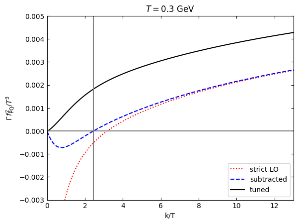
do a figure with the parameters of Fig.~3 in 2404.06113
[ ]:
k=numpy.geomspace(0.01,13,100)
plotrateleft=rate_ksvz.rate(k,1,(numpy.sqrt(4.*numpy.pi*0.310934),3.13529),0)
plotrateright=rate_ksvz.rate(k,1,(numpy.sqrt(4.*numpy.pi*0.0624043),6.),0)
[8]:
plt.rcParams['ytick.right'] = True
plt.rcParams['ytick.labelright'] = False
plt.rcParams['ytick.left'] = plt.rcParams['ytick.labelleft'] = True
plt.rcParams["xtick.top"] = True
plt.rcParams['xtick.direction']='in'
plt.rcParams['ytick.direction']='in'
plt.plot(k,plotrateleft[1],"r:",label="strict LO")
plt.plot(k,plotrateleft[2],"b--",label="subtracted")
plt.plot(k,plotrateleft[3],"k",label="tuned")
plt.xlim(0,13)
plt.ylim(-0.003,0.005)
plt.xlabel("k/T")
plt.ylabel(r"$\Gamma\,f_\mathrm{PQ}^2/T^3$")
plt.title(r'$T=0.3$ GeV')
plt.axhline(0,color='gray')
plt.axvline(numpy.sqrt(4.*numpy.pi*0.310934*(1+3.13529/6.)),color='gray')
# plt.title(r"MSSM, graviton and gravitino, SU(2) contribution only")
plt.legend()
plt.show()
plt.rcParams['ytick.right'] = True
plt.rcParams['ytick.labelright'] = False
plt.rcParams['ytick.left'] = plt.rcParams['ytick.labelleft'] = True
plt.rcParams["xtick.top"] = True
plt.rcParams['xtick.direction']='in'
plt.rcParams['ytick.direction']='in'
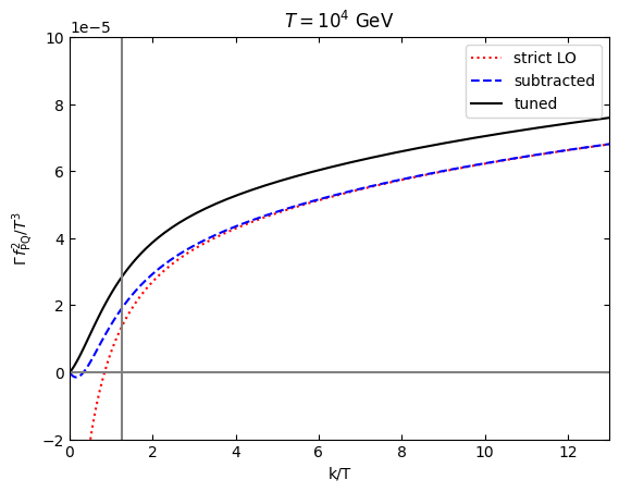
plt.plot(k,plotrateright[1],"r:",label="strict LO")
plt.plot(k,plotrateright[2],"b--",label="subtracted")
plt.plot(k,plotrateright[3],"k",label="tuned")
plt.xlim(0,13)
plt.ylim(-0.00002,0.0001)
plt.xlabel("k/T")
plt.ylabel(r"$\Gamma\,f_\mathrm{PQ}^2/T^3$")
plt.title(r'$T=10^4$ GeV')
plt.axhline(0,color='gray')
plt.axvline(numpy.sqrt(4.*numpy.pi*0.0624043*(1+1)),color='gray')
# plt.title(r"MSSM, graviton and gravitino, SU(2) contribution only")
plt.legend()
plt.show()
Numerical part with top-quark coupling, reproducing the results of 1310.6982#
In this case we want to use the most generic form of the matrix elements squared, to later consider only the \(h_t\)-proportional part
[ ]:
#create a NumRate object for the generic rate
rate_generic=NumRate(*axion_dict,1)
[10]:
axion_dict[1]
[10]:
{'gauge': ('g1', 'g2', 'g3'),
 'noneq': ('fPQ',),
 'others': ('c1', 'c2', 'c3', 'ct', 'ht')}
In order to study the contribution from the coupling to the top quark, we must set \(c_t=1\) and then also \(h_t\)=1 to rescale by the latter. The idea here is to reproduce Eq. (3.20) of 1310.6982
[11]:
from scipy.integrate import fixed_quad
def topintegrand(k):
    return k*k/(numpy.expm1(k))/(2*numpy.pi*numpy.pi)*rate_generic.rate(k,1.,(0.,0.,0.,0,0,0.,1.,1.),0)[1]
integral=fixed_quad(topintegrand,0.,20.,n=20)[0]
#put the final result in that normalization
print(integral/(3./(2.*(numpy.pi**5.))))
0.9596210947472106