Thermal moduli production

In this notebook we reproduce 2609.38151

Importing the modules

#start by importing the controller and manipulate modules
from analytical.controller import *
from numerical.manipulate import *
#reimport numpy (though it is pulled by numerical) for smarter syntax highlighting in vscode
import numpy
#import matplotlib too
import matplotlib.pyplot as plt

Field-theoretical component

The relevant part of the config file is as follows

[Model]
modelpath = /path/to/autotherm/analytical/models/moduli.fr
# Symbol for the Lagrangian in the model file
lagrangian = Ltot
# "Name" of the particle whose production rate must be computed
produced = S[2]
# List of the particles in the thermal bath (or leave empty for SM assumption)
inbath =
assumptions = Element[lambdaovermp,Reals]
replacements =
includeSM = yes
noneq = lambdaovermp
#comma-separated list of particles to be treated with a flavor expansion
flavorexpand =

moduli_dict=analytical_pipeline("../../MyModels/Moduli/moduliSM.cfg")

Let us look at this in detail. We have used the moduli-gluon Lagrangian given in (3.14) of 2609.38151

from IPython.display import display, Markdown
out=""
s = sympy.Symbol("s")
t = sympy.Symbol("t")
u = sympy.Symbol("u")
for key, item, in moduli_dict[0].items():
    sitem=sympy.simplify(sympy.sympify(item).subs(2*s*u,t*t-s*s-u*u).subs(2*s*t,u*u-s*s-t*t).subs(t*t+t*u,t*t+(s*s-t*t-u*u)/2))
    out+=f"-  $$ \\left\\vert \\mathcal{{M}}({key[0]};{key[1]},{key[2]})\\right\\vert^2={sympy.latex(sitem).replace('lambdaovermp^{2}',r'(\lambda/M_P)^2')}$$\n"
    # display(sympy.pprint(sitem))
display(Markdown(out))

• \[\left\vert \mathcal{M}(1;-1,-1)\right\vert^2=\frac{192 g_{3}^{2} (\lambda/M_P)^2 \left(t^{2} + u^{2}\right)}{s}\]
• \[\left\vert \mathcal{M}(-1;-1,1)\right\vert^2=\frac{192 g_{3}^{2} (\lambda/M_P)^2 \left(- s^{2} - u^{2}\right)}{t}\]
• \[\left\vert \mathcal{M}(-1;1,-1)\right\vert^2=\frac{192 g_{3}^{2} (\lambda/M_P)^2 \left(- s^{2} - t^{2}\right)}{u}\]
• \[\left\vert \mathcal{M}(1;1,1)\right\vert^2=\frac{48 g_{3}^{2} (\lambda/M_P)^2 \left(s^{2} + t^{2} + u^{2}\right)^{2}}{s t u}\]

Numerical part

rate_moduli=NumRate(*moduli_dict,1)

The leading-log term reads

autothermLL=rate_moduli.get_leadlog()
T = sympy.Symbol("T")
g3 = sympy.Symbol("g3")
mD = sympy.Symbol("mD")
display(Markdown(f"$$"+sympy.latex(autothermLL.subs(T*T*g3*g3,mD*mD/2)).replace('lambdaovermp^{2}',r'(\lambda/M_P)^2').replace('mD',r'm_\mathrm{D}')+f"$$"))

\[\frac{2 T (\lambda/M_P)^2 m_\mathrm{D}^{2} \log{\left(\frac{4 k^{2}}{m_\mathrm{D}^{2}} \right)}}{\pi}\]

The leading-log result given in (3.15) of 2609.38151 corresponds to multiplying this quantity by \(n_B(k)/(2\pi)^3\). Vice-versa

rateLLpaper=sympy.sympify('3*lambdaovermp^2*(2*g3^2*T^2/3)*8*T*(2*pi)^3/(32*pi^4)*log(T^2/(2*g3^2*T^2/3))')

If we take the ratio we find

rateLLpaper/autothermLL

$\displaystyle \frac{\log{\left(\frac{3}{2 g_{3}^{2}} \right)}}{\log{\left(\frac{2 k^{2}}{T^{2} g_{3}^{2}} \right)}}$

So indeed they do agree at leading log

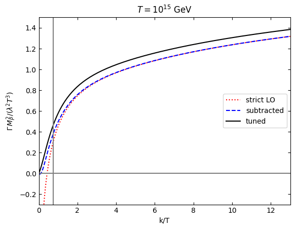
do a figure with the parameters of Fig.~3 in 2404.06113. Rescale out \((\lambda/M_P)^2\). For QCD at \(T=10^{15}\) GeV we choose, following 1911.09123, \(g_3^2\approx 0.27\).

k=numpy.geomspace(0.01,13,100)
plotrateleft=rate_moduli.rate(k,1,(numpy.sqrt(0.27),),0)

plt.rcParams['ytick.right'] = True
plt.rcParams['ytick.labelright'] = False
plt.rcParams['ytick.left'] = plt.rcParams['ytick.labelleft'] = True
plt.rcParams["xtick.top"] =  True
plt.rcParams['xtick.direction']='in'
plt.rcParams['ytick.direction']='in'
plt.plot(k,plotrateleft[1],"r:",label="strict LO")
plt.plot(k,plotrateleft[2],"b--",label="subtracted")
plt.plot(k,plotrateleft[3],"k",label="tuned")
plt.xlim(0,13)
plt.ylim(-0.3,1.5)
plt.xlabel("k/T")
plt.ylabel(r"$\Gamma\,M_P^2/(\lambda^2T^3)$")
plt.title(r'$T=10^{15}$ GeV')
plt.axhline(0,color='gray')
plt.axvline(numpy.sqrt(2*0.27),color='gray')
# plt.title(r"MSSM, graviton and gravitino, SU(2) contribution only")

plt.legend()
plt.show()

Integrate the rate in momentum to obtain the r.h.s of Eq. (3.17) in 2609.38151

from scipy.integrate import quad
def integrand(k,scheme):
    return k*k/(numpy.expm1(k))/(2*numpy.pi*numpy.pi)*rate_moduli.rate(k,1,(numpy.sqrt(0.27),),0)[scheme][0]
integralstrict=quad(integrand,0.,20.,args=(1,))[0]
integralsubtr=quad(integrand,0.,20.,args=(2,))[0]
integraltuned=quad(integrand,0.,20.,args=(3,))[0]

#put the final result in that normalization
print(integralstrict)
print(integralsubtr)
print(integraltuned)

Warning raised by the integration routine for the dim-5 t-channel subtracted for momentum 0.002714273108869958, statistics (1, 1, 1) and coefficients 1.
This is possibly not problematic. The warning message is:

The integral is probably divergent, or slowly convergent.
0.08880522470645559
0.09273871052098986
0.10223497867799197

Eq. (3.19) in 2609.38151 gives instead

0.03*(2)*0.27/(0.5**2)*6/6*8/8*numpy.log(9/(0.27*6))/numpy.log(6)

np.float64(0.06201666018722384)

which is in the right ballpark

If we use the more precise (3.18) instead we have

from scipy.special import zeta
zeta(3.)*0.27*6*8/(12*numpy.pi**3)*numpy.log(9/(0.27*6))

np.float64(0.0717979825185126)

which is closer to the LO results

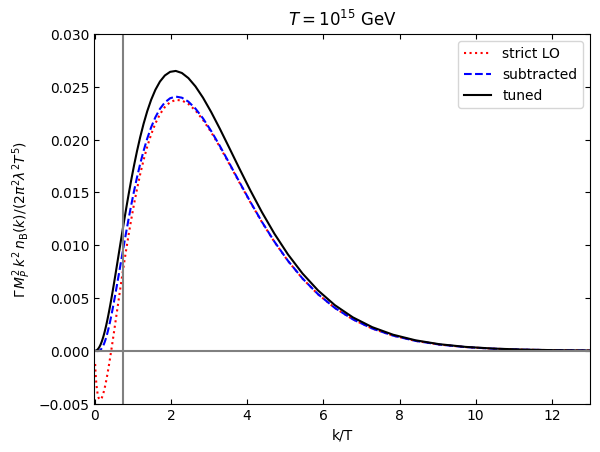
To better understand the difference between the three schemes, let us now plot the integrands for the integrals just performed

plt.rcParams['ytick.right'] = True
plt.rcParams['ytick.labelright'] = False
plt.rcParams['ytick.left'] = plt.rcParams['ytick.labelleft'] = True
plt.rcParams["xtick.top"] =  True
plt.rcParams['xtick.direction']='in'
plt.rcParams['ytick.direction']='in'
plt.plot(k,k*k/(numpy.expm1(k))/(2*numpy.pi*numpy.pi)*plotrateleft[1],"r:",label="strict LO")
plt.plot(k,k*k/(numpy.expm1(k))/(2*numpy.pi*numpy.pi)*plotrateleft[2],"b--",label="subtracted")
plt.plot(k,k*k/(numpy.expm1(k))/(2*numpy.pi*numpy.pi)*plotrateleft[3],"k",label="tuned")
plt.xlim(-0.02,13)
plt.ylim(-0.005,0.03)
plt.xlabel("k/T")
plt.ylabel(r"$\Gamma\,M_P^2\,k^2\,n_\mathrm{B}(k)/(2\pi^2\lambda^2T^5)$")
plt.title(r'$T=10^{15}$ GeV')
plt.axhline(0,color='gray')
plt.axvline(numpy.sqrt(2*0.27),color='gray')
# plt.title(r"MSSM, graviton and gravitino, SU(2) contribution only")

plt.legend()
plt.show()