Majorana Dark Matter model, reproducing the \(2\leftrightarrow 2\) part of 2012.09083#
Importing the modules#
[1]:
#start by importing the controller and manipulate modules
from analytical.controller import *
from numerical.manipulate import *
#reimport numpy (though it is pulled by numerical) for smarter syntax highlighting in vscode
import numpy
#import matplotlib too
import matplotlib.pyplot as plt
Analytical part#
The relevant part of the config file is as follows
[Model]
modelpath = /Users/jacopo/NextCloud/AUTOTHERM/autotherm/analytical/models/majoranaDM.fr
# Symbol for the Lagrangian in the model file
lagrangian = Ltot
# "Name" of the particle whose production rate must be computed
produced = F[6]
# List of the particles in the thermal bath (or leave empty for SM assumption)
inbath = S[2]+ -S[2]+
assumptions = Element[y,Reals], Element[ht,Reals], Element[lam3,Reals], Element[c1,Reals],Element[c2,Reals],Element[c3,Reals]
replacements =
includeSM = yes
noneq = y
#comma-separated list of particles to be treated with a flavor expansion
flavorexpand = {F[4],Generation}, {-F[4],Generation}
[ ]:
dm_analytical=analytical_pipeline("../../MyModels/etadm/etadm.cfg")
Numerical part#
First, we must call NumRate#
[14]:
type(dm_analytical[2])
[14]:
list
This means that the mediator has a generation-dependent thermal mass, as expected from the model. Indeed, the msq dict in dm_analytical[0] is also a list of dicts for each generation component of the exchanged mediator. Finite parts of the amplitude are assigned to each component equally. If we look at the first generation we have
[13]:
from IPython.display import display, Markdown
out=""
s = sympy.Symbol("s")
t = sympy.Symbol("t")
u = sympy.Symbol("u")
g1 = sympy.Symbol("g1")
g2 = sympy.Symbol("g2")
g3 = sympy.Symbol("g3")
ht = sympy.Symbol("ht")
y=sympy.Symbol("y")
for key, item, in dm_analytical[0][0].items():
    sitem=sympy.simplify(sympy.sympify(item).subs(2*t*u,(s*s-t*t-u*u)))
    sitemsubst= sitem
    sitemsubstcollect=0
    for exprtemp in sympy.factor(sitemsubst.expand().as_independent(ht)).subs(t+u,-s)\
        .subs(2*t*t+2*t*u,2*t*t+(s*s-t*t-u*u)).subs(t*t+2*t*u,t*t+(s*s-t*t-u*u)).subs(t*t+t*u,t*t+(s*s-t*t-u*u)/2):
        sitemsubstcollect += exprtemp.simplify()
        # beautify the output
    out+=f"- statistics: {key}:  $${sympy.latex(sitemsubstcollect).replace('ht^{2}',r'\vert h_t\vert^2')}$$\n"
    # display(sympy.pprint(sitem))
display(Markdown(out))
statistics: (1, -1, 1):
\[- \frac{2 c_{3}^{2} \vert h_t\vert^2 t y^{2}}{s} - \frac{8 y^{2} \left(g_{1}^{2} + 3 g_{3}^{2}\right) \left(3 c_{1}^{2} s^{2} + c_{1}^{2} t^{2} + c_{2}^{2} t^{2} + c_{3}^{2} t^{2}\right)}{9 s t}\]statistics: (1, 1, -1):
\[- \frac{2 c_{3}^{2} \vert h_t\vert^2 u y^{2}}{s} - \frac{8 y^{2} \left(g_{1}^{2} + 3 g_{3}^{2}\right) \left(3 c_{1}^{2} s^{2} + c_{1}^{2} u^{2} + c_{2}^{2} u^{2} + c_{3}^{2} u^{2}\right)}{9 s u}\]statistics: (-1, 1, 1):
\[\frac{8 c_{1}^{2} y^{2} \left(g_{1}^{2} + 3 g_{3}^{2}\right) \left(t^{2} + u^{2}\right)}{3 t u}\]
where we parametrized the BSM Yukawa coupling as \(y_a=y\,c_a\), with \(\sum_{a=1}^3c_a^2=1\)
If we want to just get the total matrix element squared, without caring for the decomposition in generation - which is necessary for HTL resummation - we find
[14]:
out=""
finalresult={}
for i in range(3):
    for key, item in dm_analytical[0][i].items():
        sitem=sympy.simplify(sympy.sympify(item).subs(2*t*u,(s*s-t*t-u*u)))
        sitemsubst= sitem
        sitemsubstcollect=0
        for exprtemp in sympy.factor(sitemsubst.expand().as_independent(ht)).subs(t+u,-s)\
            .subs(2*t*t+2*t*u,2*t*t+(s*s-t*t-u*u)).subs(t*t+2*t*u,t*t+(s*s-t*t-u*u)).subs(t*t+t*u,t*t+(s*s-t*t-u*u)/2):
            sitemsubstcollect += exprtemp.simplify()
        if key not in finalresult.keys():
            finalresult[key] = sitemsubstcollect
        else:
            finalresult[key] += sitemsubstcollect


c1 = sympy.Symbol("c1")
c2 = sympy.Symbol("c2")
c3 = sympy.Symbol("c3")
for key, item in finalresult.items():
    # simplify away c_2^2
    sitemsubst= item.subs(c2*c2,1-c1*c1-c3*c3)
    sitemsubstcollect=0
    for exprtemp in sympy.factor(sitemsubst.expand().as_independent(ht)).subs(t+u,-s)\
        .subs(2*t*t+2*t*u,2*t*t+(s*s-t*t-u*u)).subs(t*t+2*t*u,t*t+(s*s-t*t-u*u)).subs(t*t+t*u,t*t+(s*s-t*t-u*u)/2):
        sitemsubstcollect += exprtemp.simplify()
    # beautify the output
    out+=f"- statistics: {key}:  $${sympy.latex(sitemsubstcollect).replace('ht^{2}',r'\vert h_t\vert^2')}$$\n"
display(Markdown(out))
statistics: (1, -1, 1):
\[\frac{6 c_{3}^{2} \vert h_t\vert^2 y^{2} \left(- s^{2} - t^{2}\right)}{s t} - \frac{8 y^{2} \left(g_{1}^{2} + 3 g_{3}^{2}\right) \left(s^{2} + t^{2}\right)}{3 s t}\]statistics: (1, 1, -1):
\[\frac{6 c_{3}^{2} \vert h_t\vert^2 y^{2} \left(- s^{2} - u^{2}\right)}{s u} - \frac{8 y^{2} \left(g_{1}^{2} + 3 g_{3}^{2}\right) \left(s^{2} + u^{2}\right)}{3 s u}\]statistics: (-1, 1, 1):
\[\frac{6 c_{3}^{2} \vert h_t\vert^2 y^{2} \left(t^{2} + u^{2}\right)}{t u} + \frac{8 y^{2} \left(g_{1}^{2} + 3 g_{3}^{2}\right) \left(t^{2} + u^{2}\right)}{3 t u}\]
In this case iterate_decomposition needs to be called for each subset of matrix elements squared and masses, corresponding to the contribution of each \(u_{Ri}\), where \(i\) denotes the generation of the up-type right-handed quark
[15]:
rate_dm=[NumRate(dm_analytical[0][i],dm_analytical[1],dm_analytical[2][i],1) for i in range(0,len(dm_analytical[0]))]
/var/folders/fd/k76vq6lj73v570m2x2k93yvm0000gp/T/ipykernel_65811/902009786.py:1: AutothermWarning: The ratio between the fermion mass g1**2/9 + g3**2/3 and the coefficient of the IR divergence 4*pi**2*c1**2*g1**2/3 + 4*pi**2*c1**2*g3**2 depends on the coupling constants entering the mass.
This is most likely not problematic, continuing with evaluation.
  rate_dm=[NumRate(dm_analytical[0][i],dm_analytical[1],dm_analytical[2][i],1) for i in range(0,len(dm_analytical[0]))]
/var/folders/fd/k76vq6lj73v570m2x2k93yvm0000gp/T/ipykernel_65811/902009786.py:1: AutothermWarning: The ratio between the fermion mass g1**2/9 + g3**2/3 and the coefficient of the IR divergence 4*pi**2*c2**2*g1**2/3 + 4*pi**2*c2**2*g3**2 depends on the coupling constants entering the mass.
This is most likely not problematic, continuing with evaluation.
  rate_dm=[NumRate(dm_analytical[0][i],dm_analytical[1],dm_analytical[2][i],1) for i in range(0,len(dm_analytical[0]))]
/var/folders/fd/k76vq6lj73v570m2x2k93yvm0000gp/T/ipykernel_65811/902009786.py:1: AutothermWarning: The ratio between the fermion mass g1**2/9 + g3**2/3 + ht**2/4 and the coefficient of the IR divergence 4*pi**2*c3**2*g1**2/3 + 4*pi**2*c3**2*g3**2 + 3*pi**2*c3**2*ht**2 depends on the coupling constants entering the mass.
This is most likely not problematic, continuing with evaluation.
  rate_dm=[NumRate(dm_analytical[0][i],dm_analytical[1],dm_analytical[2][i],1) for i in range(0,len(dm_analytical[0]))]
The leading-log term reads
[16]:
leadlog=sum([contrib.get_leadlog() for contrib in rate_dm]).simplify()
leadlog
[16]:
reexpress this in terms of the generations and their asymptotic masses for the \(u_R\)
[34]:
md1 = sympy.Symbol(r"m_{\infty 1}^2")
md2 = sympy.Symbol(r"m_{\infty 2}^2")
md3 = sympy.Symbol(r"m_{\infty 3}^2")
T = sympy.S("T")
k= sympy.S("k")
nB= sympy.Function("n_B")
llsimple=0
llsimple += leadlog.subs(c2,0).subs(c3,0).subs(g3*g3,3*(md1/T/T-g1*g1/9)).simplify()
llsimple += leadlog.subs(c1,0).subs(c3,0).subs(g3*g3,3*(md2/T/T-g1*g1/9)).simplify()
llsimple += leadlog.subs(c2,0).subs(c1,0).subs(g3*g3,3*(md3/T/T-g1*g1/9-ht*ht/4)).simplify()
llsimple.subs(sympy.tanh(k/(2*T)),1/(1+2* nB(k))).simplify()
[34]:
Prepare to compare with the known determination extracted from 2012.09083. overallt and overallu denote the top and up/charm contributions respectively
[17]:
overallt=sympy.S("4*3/2*y^2*(4/9*g1^2+4/3*g3^2+ht^2)")
FIMPdictt = {(-1,1,1):str(overallt*sympy.S("(t/u+u/t)")),\
             (1,-1,1):str(overallt*sympy.S("(-t/s-s/t)")),\
              (1,1,-1):str(overallt*sympy.S("(-u/s-s/u)"))}
testFIMPt = NumRate(FIMPdictt, {"noneq": ("y",),  "gauge": ("g1","g3"),"others" : ("ht",)}, "(1/9*g1^2+1/3*g3^2+ht^2/4)",1)
overallu=sympy.S("4*3/2*y^2*(4/9*g1^2+4/3*g3^2)")
FIMPdictu = {(-1,1,1):str(overallu*sympy.S("(t/u+u/t)")),\
             (1,-1,1):str(overallu*sympy.S("(-t/s-s/t)")),\
              (1,1,-1):str(overallu*sympy.S("(-u/s-s/u)"))}
testFIMPu = NumRate(FIMPdictu, {"noneq": ("y",),  "gauge": ("g1","g3"),"others" : ("ht",)}, "(1/9*g1^2+1/3*g3^2)",1)
Start by fixing \(c_i=1/\sqrt{3}\), i.e. the \(\chi\) fermion couples equally to all three generations.
[7]:
dm_analytical[1]
[7]:
{'gauge': ('g1', 'g3'), 'noneq': ('y',), 'others': ('c1', 'c2', 'c3', 'ht')}
[18]:
testrate=[]
for i in range (0,3):
    testrate.append(rate_dm[i].rate(1.,1,(0.1,0.1,1/numpy.sqrt(3),1/numpy.sqrt(3),1/numpy.sqrt(3),0.1),0))
for i in range(1,4):
    print(testrate[0][i]+testrate[1][i]+testrate[2][i])
[0.00208345865212976]
[0.00208393041945224]
[0.00209239323829194]
[19]:
urate=testFIMPu.rate(1.,1.,(0.1,0.1,0.1),0)
trate=testFIMPt.rate(1.,1.,(0.1,0.1,0.1),0)
for i in range(1,4):
    print(2/3*urate[i]+1/3*trate[i])
[0.00208345865185283]
[0.00208393041917532]
[0.00209239324073410]
Now consider \(c_1=c_2=1/\sqrt{2}\), \(c_3=0\), i.e. the \(\chi\) fermion couples only to the \(u\) and \(c\) quarks
[20]:
testrate=[]
for i in range (0,3):
    testrate.append(rate_dm[i].rate(1.,1,(0.1,0.1,1/numpy.sqrt(2),1/numpy.sqrt(2),0,0.1),0))
for i in range(1,4):
    print(testrate[0][i]+testrate[1][i]+testrate[2][i])
[0.00181066949987032]
[0.00181098821532267]
[0.00181753896558478]
[9]:
urate[1:]
[9]:
[array([0.00181066949732706], dtype=object),
 array([0.00181098821277941], dtype=object),
 array([0.00181753897645469], dtype=object)]
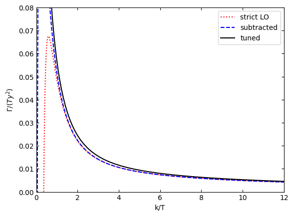
do a figure with the parameters of Fig.~8 in 2012.09083
[21]:
plotrate=[]
k=numpy.logspace(-2,numpy.log10(12),100,10)
for i in range (0,3):
    plotrate.append(rate_dm[i].rate(k,1,(0.,numpy.sqrt(0.85),0.,0.,1.,numpy.sqrt(0.6)),0))
totratestrict=plotrate[0][1]+plotrate[1][1]+plotrate[2][1]
totratesubtr=plotrate[0][2]+plotrate[1][2]+plotrate[2][2]
totratetuned=plotrate[0][3]+plotrate[1][3]+plotrate[2][3]
[11]:
plt.rcParams['ytick.right'] = True
plt.rcParams['ytick.labelright'] = False
plt.rcParams['ytick.left'] = plt.rcParams['ytick.labelleft'] = True
plt.rcParams["xtick.top"] =  True
plt.rcParams['xtick.direction']='in'
plt.rcParams['ytick.direction']='in'
plt.plot(k,totratestrict,"r:",label="strict LO")
plt.plot(k,totratesubtr,"b--",label="subtracted")
plt.plot(k,totratetuned,"k",label="tuned")
plt.xlim(0,12)
plt.ylim(-0.0,0.08)
plt.xlabel("k/T")
plt.ylabel(r"$\Gamma/(Ty^2)$")
# plt.title(r"MSSM, graviton and gravitino, SU(2) contribution only")

plt.legend()
plt.show()
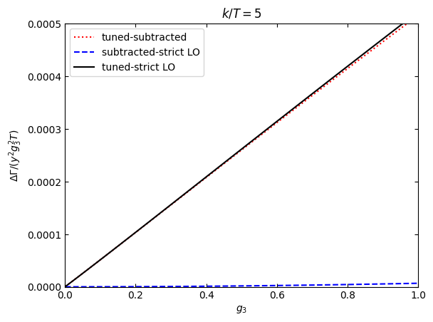
Now we fix \(k/T\) and do a plot where we set \(h_t=g_1=0\) and explore the small \(g_3\) limit, so as to show how the three rates differ
[56]:
myk=5
ngs=100
gvec=numpy.logspace(-3,0,ngs)
lovec=numpy.zeros(ngs)
subtrvec=numpy.zeros(ngs)
tunedvec=numpy.zeros(ngs)
for j in range(ngs):
    for i in range (0,3):
        temprate=rate_dm[i].rate(myk,1,(0.,gvec[j],0.,0.,1.,0.),0)
        lovec[j] +=temprate[1][0]
        subtrvec[j] +=temprate[2][0]
        tunedvec[j] +=temprate[3][0]
[57]:
plt.rcParams['ytick.right'] = True
plt.rcParams['ytick.labelright'] = False
plt.rcParams['ytick.left'] = plt.rcParams['ytick.labelleft'] = True
plt.rcParams["xtick.top"] =  True
plt.rcParams['xtick.direction']='in'
plt.rcParams['ytick.direction']='in'
plt.plot(gvec,(tunedvec-subtrvec)/gvec**2,"r:",label="tuned-subtracted")
plt.plot(gvec,(subtrvec-lovec)/gvec**2,"b--",label="subtracted-strict LO")
plt.plot(gvec,(tunedvec-lovec)/gvec**2,"k",label="tuned-strict LO")
plt.legend()
plt.xlim(0,1)
plt.ylim(0,0.0005)
plt.xlabel(r'$g_3$')
plt.ylabel(r"$\Delta\Gamma/(y^2g_3^2 T)$")
plt.title(r'$k/T=$'+str(myk))
plt.show()
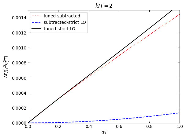
do the same for \(k/T=2\)
[54]:
myk2=2
ngs=100
gvec=numpy.logspace(-3,0,ngs)
lovec2=numpy.zeros(ngs)
subtrvec2=numpy.zeros(ngs)
tunedvec2=numpy.zeros(ngs)
for j in range(ngs):
    for i in range (0,3):
        temprate=rate_dm[i].rate(myk2,1,(0.,gvec[j],0.,0.,1.,0.),0)
        lovec2[j] +=temprate[1][0]
        subtrvec2[j] +=temprate[2][0]
        tunedvec2[j] +=temprate[3][0]
[55]:
plt.rcParams['ytick.right'] = True
plt.rcParams['ytick.labelright'] = False
plt.rcParams['ytick.left'] = plt.rcParams['ytick.labelleft'] = True
plt.rcParams["xtick.top"] =  True
plt.rcParams['xtick.direction']='in'
plt.rcParams['ytick.direction']='in'
plt.plot(gvec,(tunedvec2-subtrvec2)/gvec**2,"r:",label="tuned-subtracted")
plt.plot(gvec,(subtrvec2-lovec2)/gvec**2,"b--",label="subtracted-strict LO")
plt.plot(gvec,(tunedvec2-lovec2)/gvec**2,"k",label="tuned-strict LO")
plt.legend()
plt.xlim(0,1)
plt.ylim(0,0.0015)
plt.xlabel(r'$g_3$')
plt.ylabel(r"$\Delta\Gamma/(y^2g_3^2 T)$")
plt.title(r'$k/T=$'+str(myk2))
plt.show()